Advertisement
 20:46
20:46
Integration and the fundamental theorem of calculus | Chapter 8, Essence of calculus
3Blue1Brown
·
May 12, 2026
Open on YouTube
Transcript
0:12
This guy, Grothendieck, is somewhat of a mathematical idol to me,
0:15
and I just love this quote, don't you?
0:18
Too often in math, we dive into showing that a certain fact is true
0:22
with a long series of formulas before stepping back and making sure it feels reasonable,
0:27
and preferably obvious, at least at an intuitive level.
0:31
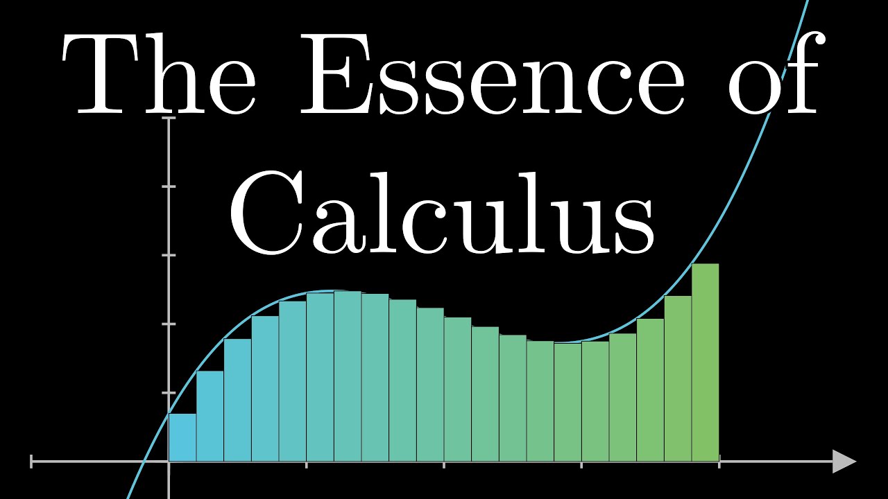
In this video, I want to talk about integrals,
0:33
and the thing that I want to become almost obvious is that they are an
0:37
inverse of derivatives.
Advertisement
0:39
Here we're just going to focus on one example,
0:42
which is a kind of dual to the example of a moving car that I talked about in chapter
0:46
2 of the series, introducing derivatives.
0:49
Then in the next video we're going to see how this same idea generalizes,
0:52
but to a couple other contexts.
0:55
Imagine you're sitting in a car, and you can't see out the window,
0:58
all you see is the speedometer.
1:02
At some point the car starts moving, speeds up,
1:05
and then slows back down to a stop, all over the course of 8 seconds.
1:11
The question is, is there a nice way to figure out how far you've
Advertisement
1:15
travelled during that time based only on your view of the speedometer?
1:19
Or better yet, can you find a distance function, s of t,
1:23
that tells you how far you've travelled after a given amount of time, t,
1:27
somewhere between 0 and 8 seconds?
1:30
Let's say you take note of the velocity at every second,
1:34
and make a plot over time that looks something like this.
1:38
And maybe you find that a nice function to model that velocity
1:43
over time in meters per second is v of t equals t times 8 minus t.
1:48
You might remember, in chapter 2 of this series we were looking at
1:51
the opposite situation, where you knew what a distance function was,
1:55
s of t, and you wanted to figure out the velocity function from that.
1:59
There I showed how the derivative of a distance vs.
2:02
time function gives you a velocity vs.
2:04
time function.
2:06
So in our current situation, where all we know is velocity,
2:09
it should make sense that finding a distance vs.
2:12
time function is going to come down to asking what
2:15
function has a derivative of t times 8 minus t.
2:19
This is often described as finding the antiderivative of a function, and indeed,
2:23
that's what we'll end up doing, and you could even pause right now and try that.
2:27
But first, I want to spend the bulk of this video showing how this question is related
2:32
to finding the area bounded by the velocity graph,
2:35
because that helps to build an intuition for a whole class of problems,
2:39
things called integral problems in math and science.
2:42
To start off, notice that this question would be a lot easier
2:45
if the car was just moving at a constant velocity, right?
2:49
In that case, you could just multiply the velocity in meters per second times the amount
2:54
of time that has passed in seconds, and that would give you the number of meters traveled.
3:00
And notice, you can visualize that product, that distance, as an area.
3:05
And if visualizing distance as area seems kind of weird, I'm right there with you.
3:08
It's just that on this plot, where the horizontal direction has units of seconds,
3:13
and the vertical direction has units of meters per second,
3:17
units of area just very naturally correspond to meters.
3:22
But what makes our situation hard is that velocity is not constant,
3:25
it's incessantly changing at every single instant.
3:30
It would even be a lot easier if it only ever changed at a handful of points,
3:35
maybe staying static for the first second, and then suddenly discontinuously
3:39
jumping to a constant 7 meters per second for the next second, and so on,
3:43
with discontinuous jumps to portions of constant velocity.
3:48
That would make it uncomfortable for the driver,
3:51
in fact it's actually physically impossible, but it would make your calculations
3:55
a lot more straightforward.
3:57
You could just compute the distance traveled on each interval by multiplying the constant
4:02
velocity on that interval by the change in time, and then just add all of those up.
4:09
So what we're going to do is approximate the velocity function as if it
4:13
was constant on a bunch of intervals, and then, as is common in calculus,
4:17
we'll see how refining that approximation leads us to something more precise.
4:24
Here, let's make this a little more concrete by throwing in some numbers.
4:28
Chop up the time axis between 0 and 8 seconds into many small intervals,
4:33
each with some little width dt, something like 0.25 seconds.
4:38
Consider one of those intervals, like the one between t equals 1 and 1.25.
4:45
In reality, the car speeds up from 7 m per second to about 8.4 m per
4:49
second during that time, and you could find those numbers just by
4:53
plugging in t equals 1 and t equals 1.25 to the equation for velocity.
4:59
What we want to do is approximate the car's motion
5:02
as if its velocity was constant on that interval.
5:05
Again, the reason for doing that is we don't really know
5:08
how to handle situations other than constant velocity ones.
5:13
You could choose this constant to be anything between 7 and 8.4.
5:18
It actually doesn't matter.
5:20
All that matters is that our sequence of approximations,
5:23
whatever they are, gets better and better as dt gets smaller and smaller.
5:28
That treating this car's journey as a bunch of discontinuous jumps
5:32
in speed between portions of constant velocity becomes a less-wrong
5:36
reflection of reality as we decrease the time between those jumps.
5:42
So for convenience, on an interval like this, let's just approximate the
5:46
speed with whatever the true car's velocity is at the start of that interval,
5:50
the height of the graph above the left side, which in this case is 7.
5:55
In this example interval, according to our approximation,
6:00
the car moves 7 m per second times 0.25 seconds.
6:04
That's 1.75 meters, and it's nicely visualized as the area of this thin rectangle.
6:10
In truth, that's a little under the real distance traveled, but not by much.
6:14
The same goes for every other interval.
6:17
The approximated distance is v of t times dt, it's just that you'd be plugging in a
6:22
different value for t at each one of these, giving a different height for each rectangle.
6:29
I'm going to write out an expression for the sum of
6:32
the areas of all those rectangles in kind of a funny way.
6:36
Take this symbol here, which looks like a stretched s for sum,
6:40
and put a 0 at its bottom and an 8 at its top,
6:43
to indicate that we'll be ranging over time steps between 0 and 8 seconds.
6:48
And as I said, the amount we're adding up at each time step is v of t times dt.
6:55
Two things are implicit in this notation.
6:58
First of all, that value dt plays two separate roles.
7:01
Not only is it a factor in each quantity we're adding up,
7:05
it also indicates the spacing between each sampled time step.
7:09
So when you make dt smaller and smaller, even though it decreases the area of
7:13
each rectangle, it increases the total number of rectangles whose areas we're adding up,
7:18
because if they're thinner, it takes more of them to fill that space.
7:22
And second, the reason we don't use the usual sigma notation to indicate a sum is that
7:28
this expression is technically not any particular sum for any particular choice of dt.
7:33
It's meant to express whatever that sum approaches as dt approaches 0.
7:39
And as you can see, what that approaches is the
7:42
area bounded by this curve and the horizontal axis.
7:46
Remember, smaller choices of dt indicate closer approximations for the original question,
7:51
how far does the car actually go?
7:54
So this limiting value for the sum, the area under this curve,
7:58
gives us the precise answer to the question in full unapproximated precision.
8:04
Now tell me that's not surprising.
8:06
We had this pretty complicated idea of approximations that
8:09
can involve adding up a huge number of very tiny things.
8:13
And yet, the value that those approximations approach can be described so simply,
8:18
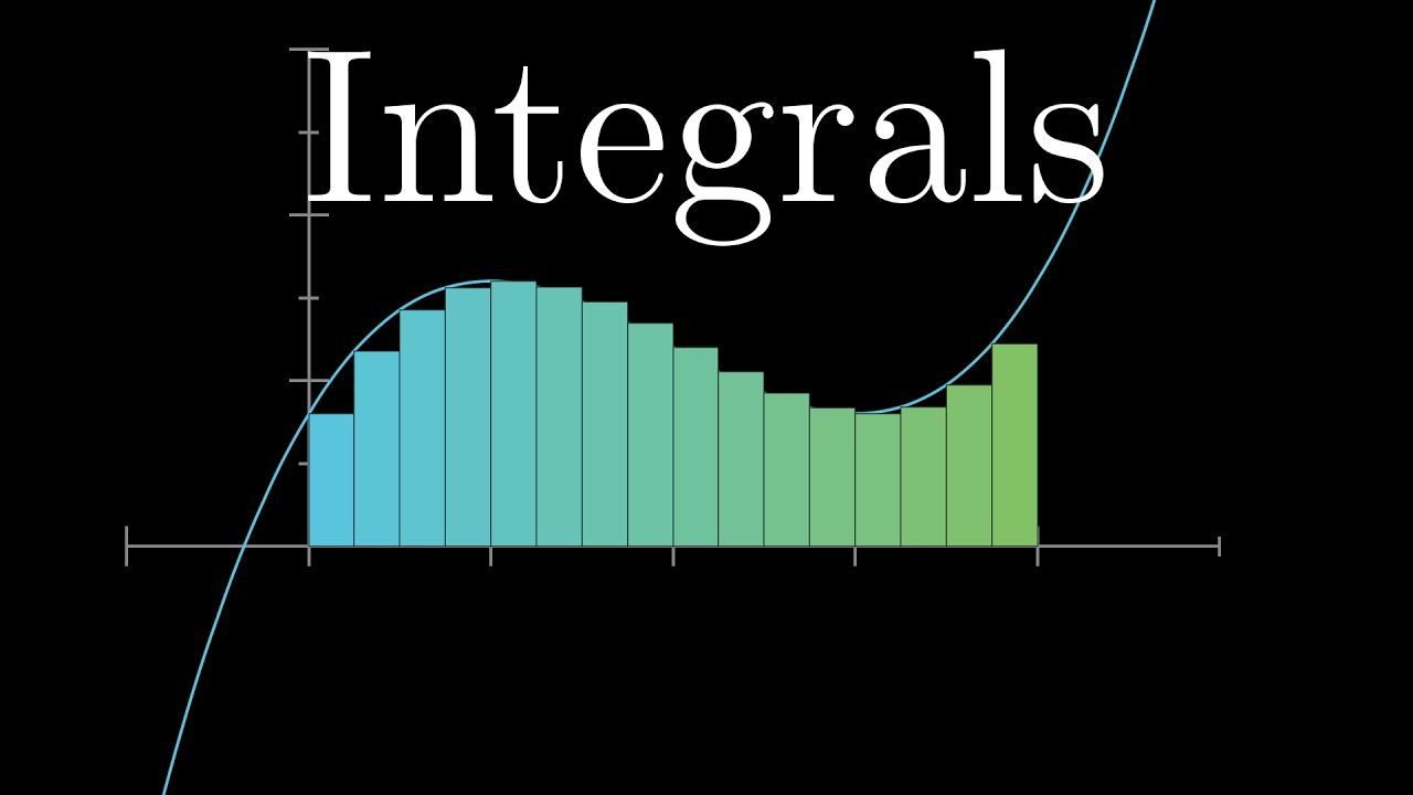
it's just the area underneath this curve.
8:22
This expression is called an integral of v of t,
8:25
since it brings all of its values together, it integrates them.
8:30
Now at this point, you could say, how does this help?
8:33
You've just reframed one hard question, finding how far the car has traveled,
8:37
into an equally hard problem, finding the area between this graph and the horizontal axis.
8:43
And you'd be right.
8:45
If the velocity-distance duo was the only thing we cared about, most of this video,
8:50
with all the area under a curve nonsense, would be a waste of time.
8:54
We could just skip straight ahead to finding an antiderivative.
8:58
But finding the area between a function's graph and the horizontal axis
9:02
is somewhat of a common language for many disparate problems that can be
9:06
broken down and approximated as the sum of a large number of small things.
9:12
You'll see more in the next video, but for now I'll just say in
9:15
the abstract that understanding how to interpret and how to
9:19
compute the area under a graph is a very general problem-solving tool.
9:23
In fact, the first video of this series already covered the basics of how this works,
9:28
but now that we have more of a background with derivatives,
9:31
we can take this idea to its completion.
9:34
For a velocity example, think of this right endpoint as a variable, capital T.
9:41
So we're thinking of this integral of the velocity function between 0 and T,
9:45
the area under this curve between those inputs,
9:48
as a function where the upper bound is the variable.
9:52
That area represents the distance the car has travelled after T seconds, right?
9:57
So in reality, this is a distance vs.
9:59
time function, s of t.
10:01
Now ask yourself, what is the derivative of that function?
10:07
On the one hand, a tiny change in distance over a tiny change in time is velocity,
10:12
that is what velocity means.
10:14
But there's another way to see this, purely in terms of this graph and this area,
10:19
which generalizes a lot better to other integral problems.
10:23
A slight nudge of dt to the input causes that area to increase,
10:27
some little ds represented by the area of this sliver.
10:32
The height of that sliver is the height of the graph at that point,
10:37
v of t, and its width is dt.
10:39
And for small enough dt, we can basically consider that sliver to be a rectangle,
10:45
so this little bit of added area, ds, is approximately equal to v of t times dt.
10:51
And because that's an approximation that gets better and better for smaller dt,
10:56
the derivative of that area function, ds, dt, at this point equals vt,
11:01
the value of the velocity function at whatever time we started on.
11:06
And that right there is a super general argument.
11:09
The derivative of any function giving the area under a
11:12
graph like this is equal to the function for the graph itself.
11:18
So, if our velocity function is t times 8-t, what should s be?
11:25
What function of t has a derivative of t times 8-t?
11:30
It's easier to see if we expand this out, writing it as 8t minus t squared,
11:34
and then we can just take each part one at a time.
11:37
What function has a derivative of 8t?
11:42
We know that the derivative of t squared is 2t,
11:45
so if we just scale that up by a factor of 4, we can see that the derivative
11:50
of 4t squared is 8t.
11:53
And for that second part, what kind of function do
11:55
you think might have negative t squared as a derivative?
12:00
Using the power rule again, we know that the derivative of a cubic term,
12:04
t cubed, gives us a square term, 3t squared.
12:08
So if we just scale that down by a third, the
12:11
derivative of 1 third t cubed is exactly t squared.
12:14
And then making that negative, we'd see that negative
12:17
1 third t cubed has a derivative of negative t squared.
12:22
Therefore, the antiderivative of our function,
12:26
8t minus t squared, is 4t squared minus 1 third t cubed.
12:32
But there's a slight issue here.
12:34
We could add any constant we want to this function,
12:37
and its derivative is still 8t minus t squared.
12:41
The derivative of a constant always goes to zero.
12:45
And if you were to graph s of t, you could think of this in the sense that moving a
12:49
graph of a distance function up and down does nothing to affect its slope at every input.
12:54
So in reality, there's actually infinitely many different
12:58
possible antiderivative functions, and every one of them looks
13:02
like 4t squared minus 1 third t cubed plus c, for some constant c.
13:08
But there is one piece of information we haven't used yet that will let
13:12
us zero in on which antiderivative to use, the lower bound of the integral.
13:18
This integral has to be zero when we drag that right
13:21
endpoint all the way to the left endpoint, right?
13:24
The distance travelled by the car between 0 seconds and 0 seconds is… well, zero.
13:31
So as we found, the area as a function of capital
13:34
T is an antiderivative for the stuff inside.
13:38
And to choose what constant to add to this expression,
13:42
you subtract off the value of that antiderivative function at the lower bound.
13:48
If you think about it for a moment, that ensures that the
13:51
integral from the lower bound to itself will indeed be zero.
13:57
As it so happens, when you evaluate the function we have here at t equals zero,
14:02
you get zero.
14:03
So in this specific case, you don't need to subtract anything off.
14:07
For example, the total distance travelled during the full 8 seconds
14:13
is this expression evaluated at t equals 8, which is 85.33 minus 0.
14:18
So the answer as a whole is 85.33.
14:23
But a more typical example would be something like the integral between 1 and 7.
14:28
That's the area pictured here, and it represents
14:30
the distance travelled between 1 second and 7 seconds.
14:36
What you do is evaluate the antiderivative we found at the top bound,
14:41
7, and subtract off its value at the bottom bound, 1.
14:45
Notice, by the way, it doesn't matter which antiderivative we chose here.
14:50
If for some reason it had a constant added to it, like 5, that constant would cancel out.
14:58
More generally, any time you want to integrate some function, and remember,
15:03
you think of that as adding up values f of x times dx for inputs in a certain range,
15:08
and then asking what is that sum approach as dx approaches 0.
15:13
The first step to evaluating that integral is to find an antiderivative,
15:18
some other function, capital F, whose derivative is the thing inside the integral.
15:24
Then the integral equals this antiderivative evaluated
15:28
at the top bound minus its value at the bottom bound.
15:32
And this fact right here that you're staring at is the fundamental theorem of calculus.
15:38
And I want you to appreciate something kind of crazy about this fact.
15:41
The integral, the limiting value for the sum of all these thin rectangles,
15:46
takes into account every single input on the continuum,
15:49
from the lower bound to the upper bound.
15:52
That's why we use the word integrate, it brings them all together.
15:56
And yet, to actually compute it using an antiderivative,
16:00
you only look at two inputs, the top bound and the bottom bound.
16:05
It almost feels like cheating.
16:06
Finding the antiderivative implicitly accounts for all the
16:10
information needed to add up the values between those two bounds.
16:15
That's just crazy to me.
16:18
This idea is deep, and there's a lot packed into this whole concept,
16:22
so let's recap everything that just happened, shall we?
16:26
We wanted to figure out how far a car goes just by looking at the speedometer.
16:31
And what makes that hard is that velocity is always changing.
16:35
If you approximate velocity to be constant on multiple different intervals,
16:39
you could figure out how far the car goes on each interval with multiplication,
16:43
and then add all of those up.
16:46
Better and better approximations for the original problem correspond to
16:50
collections of rectangles whose aggregate area is closer and closer to
16:54
being the area under this curve between the start time and the end time.
16:58
So that area under the curve is actually the precise distance
17:03
traveled for the true nowhere constant velocity function.
17:08
If you think of that area as a function itself,
17:11
with a variable right endpoint, you can deduce that the derivative
17:15
of that area function must equal the height of the graph at every point.
17:21
And that's really the key right there.
17:22
It means that to find a function giving this area,
17:26
you ask, what function has v of t as a derivative?
17:30
There are actually infinitely many antiderivatives of a given function,
17:34
since you can always just add some constant without affecting the derivative,
17:38
so you account for that by subtracting off the value of whatever antiderivative function
17:43
you choose at the bottom bound.
17:46
By the way, one important thing to bring up before we leave is the idea of negative area.
17:53
What if the velocity function was negative at some point, meaning the car goes backwards?
17:58
It's still true that a tiny distance traveled ds on a little time interval is
18:03
about equal to the velocity at that time multiplied by the tiny change in time.
18:08
It's just that the number you'd plug in for velocity would be negative,
18:13
so the tiny change in distance is negative.
18:16
In terms of our thin rectangles, if a rectangle goes below the horizontal axis,
18:21
like this, its area represents a bit of distance traveled backwards,
18:25
so if what you want in the end is to find a distance between the car's
18:29
start point and its end point, this is something you'll want to subtract.
18:35
And that's generally true of integrals.
18:37
Whenever a graph dips below the horizontal axis,
18:40
the area between that portion of the graph and the horizontal axis is counted as negative.
18:46
What you'll commonly hear is that integrals don't measure area per se,
18:50
they measure the signed area between the graph and the horizontal axis.
18:55
Next up, I'm going to bring up more context where this idea
18:58
of an integral and area under curves comes up,
19:01
along with some other intuitions for this fundamental theorem of calculus.
19:06
Maybe you remember, chapter 2 of this series introducing the derivative
19:10
was sponsored by The Art of Problem Solving, so I think there's
19:13
something elegant to the fact that this video, which is kind of a duel to that one,
19:18
was also supported in part by The Art of Problem Solving.
19:22
I really can't imagine a better sponsor for this channel,
19:25
because it's a company whose books and courses I recommend to people anyway.
19:29
They were highly influential to me when I was a student developing a love for
19:33
creative math, so if you're a parent looking to foster your own child's love
19:37
for the subject, or if you're a student who wants to see what math has to offer
19:42
beyond rote schoolwork, I cannot recommend The Art of Problem Solving enough.
19:46
Whether that's their newest development to build the right intuitions in
19:50
elementary school kids, called Beast Academy, or their courses in higher-level
19:55
topics and contest preparation, going to aops.com slash 3blue1brown,
19:59
or clicking on the link in the description, lets them know you came from this channel,
20:04
which may encourage them to support future projects like this one.
20:08
I consider these videos a success not when they teach people a particular bit of math,
20:13
which can only ever be a drop in the ocean, but when they encourage people
20:17
to go and explore that expanse for themselves,
20:20
and The Art of Problem Solving is among the few great places to actually do
20:24
that exploration.
— end of transcript —
Advertisement