Advertisement
 17:04
17:04
Transcript
0:14
Hey everyone, Grant here.
0:16
This is the first video in a series on the essence of calculus,
0:19
and I'll be publishing the following videos once per day for the next 10 days.
0:24
The goal here, as the name suggests, is to really get
0:26
the heart of the subject out in one binge-watchable set.
0:30
But with a topic that's as broad as calculus, there's a lot of things that can mean,
0:34
so here's what I have in mind specifically.
0:36
Calculus has a lot of rules and formulas which
Advertisement
0:39
are often presented as things to be memorized.
0:42
Lots of derivative formulas, the product rule, the chain rule,
0:45
implicit differentiation, the fact that integrals and derivatives are opposite,
0:49
Taylor series, just a lot of things like that.
0:52
And my goal is for you to come away feeling like
0:55
you could have invented calculus yourself.
0:57
That is, cover all those core ideas, but in a way that makes clear where they
1:01
actually come from, and what they really mean, using an all-around visual approach.
1:06
Inventing math is no joke, and there is a difference between being
1:10
told why something's true, and actually generating it from scratch.
Advertisement
1:14
But at all points, I want you to think to yourself, if you were an early mathematician,
1:19
pondering these ideas and drawing out the right diagrams,
1:22
does it feel reasonable that you could have stumbled across these truths yourself?
1:26
In this initial video, I want to show how you might stumble into the core ideas of
1:31
calculus by thinking very deeply about one specific bit of geometry,
1:35
the area of a circle.
1:37
Maybe you know that this is pi times its radius squared, but why?
1:41
Is there a nice way to think about where this formula comes from?
1:45
Well, contemplating this problem and leaving yourself open to exploring the
1:49
interesting thoughts that come about can actually lead you to a glimpse of three
1:53
big ideas in calculus, integrals, derivatives, and the fact that they're opposites.
1:59
But the story starts more simply, just you and a circle, let's say with radius 3.
2:05
You're trying to figure out its area, and after going through a lot of
2:09
paper trying different ways to chop up and rearrange the pieces of that area,
2:13
many of which might lead to their own interesting observations,
2:16
maybe you try out the idea of slicing up the circle into many concentric rings.
2:22
This should seem promising because it respects the symmetry of the circle,
2:25
and math has a tendency to reward you when you respect its symmetries.
2:30
Let's take one of those rings, which has some inner radius r that's between 0 and 3.
2:36
If we can find a nice expression for the area of each ring like this one,
2:39
and if we have a nice way to add them all up,
2:42
it might lead us to an understanding of the full circle's area.
2:46
Maybe you start by imagining straightening out this ring.
2:50
And you could try thinking through exactly what this new shape is and what its
2:54
area should be, but for simplicity, let's just approximate it as a rectangle.
3:00
The width of that rectangle is the circumference of the original ring,
3:03
which is 2 pi times r, right?
3:05
I mean, that's essentially the definition of pi.
3:08
And its thickness?
3:10
Well, that depends on how finely you chopped up the circle in the first place,
3:14
which was kind of arbitrary.
3:16
In the spirit of using what will come to be standard calculus notation,
3:20
let's call that thickness dr for a tiny difference in the radius from one ring to
3:24
the next.
3:25
Maybe you think of it as something like 0.1.
3:28
So approximating this unwrapped ring as a thin rectangle,
3:32
its area is 2 pi times r, the radius, times dr, the little thickness.
3:38
And even though that's not perfect, for smaller and smaller choices of dr,
3:42
this is actually going to be a better and better approximation for that area,
3:46
since the top and the bottom sides of this shape are going to get closer and closer to
3:50
being exactly the same length.
3:53
So let's just move forward with this approximation,
3:55
keeping in the back of our minds that it's slightly wrong,
3:58
but it's going to become more accurate for smaller and smaller choices of dr.
4:03
That is, if we slice up the circle into thinner and thinner rings.
4:07
So just to sum up where we are, you've broken up the area of the circle into
4:12
all of these rings, and you're approximating the area of each one of those as
4:17
2 pi times its radius times dr, where the specific value for that inner radius
4:22
ranges from 0 for the smallest ring up to just under 3 for the biggest ring,
4:26
spaced out by whatever the thickness is that you choose for dr, something like 0.1.
4:33
And notice that the spacing between the values here corresponds to the
4:36
thickness dr of each ring, the difference in radius from one ring to the next.
4:42
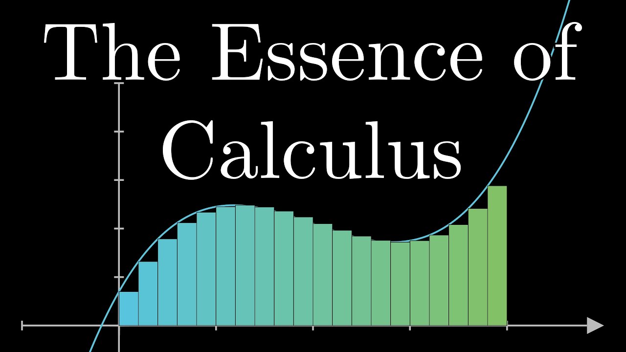
In fact, a nice way to think about the rectangles approximating each
4:46
ring's area is to fit them all upright side by side along this axis.
4:50
Each one has a thickness dr, which is why they fit so snugly right there together,
4:55
and the height of any one of these rectangles sitting above some specific value of r,
5:01
like 0.6, is exactly 2 pi times that value.
5:04
That's the circumference of the corresponding ring that this rectangle approximates.
5:09
Pictures like this 2 pi r can get tall for the screen,
5:12
I mean 2 times pi times 3 is around 19, so let's just throw up a y axis that's
5:16
scaled a little differently so that we can actually fit all of these rectangles
5:21
on the screen.
5:23
A nice way to think about this setup is to draw the graph of 2 pi r,
5:26
which is a straight line that has a slope 2 pi.
5:30
Each of these rectangles extends up to the point where it just barely touches that graph.
5:36
Again, we're being approximate here.
5:37
Each of these rectangles only approximates the
5:40
area of the corresponding ring from the circle.
5:42
But remember, that approximation, 2 pi r times dr,
5:46
gets less and less wrong as the size of dr gets smaller and smaller.
5:51
And this has a very beautiful meaning when we're
5:53
looking at the sum of the areas of all those rectangles.
5:57
For smaller and smaller choices of dr, you might at first
6:00
think that turns the problem into a monstrously large sum.
6:03
I mean, there's many many rectangles to consider,
6:05
and the decimal precision of each one of their areas is going to be an
6:08
absolute nightmare.
6:10
But notice, all of their areas in aggregate just looks like the area under a graph.
6:15
And that portion under the graph is just a triangle,
6:19
a triangle with a base of 3 and a height that's 2 pi times 3.
6:24
So its area, 1 half base times height, works out to be exactly pi times 3 squared.
6:31
Or if the radius of our original circle was some other value,
6:35
capital R, that area comes out to be pi times r squared.
6:39
And that's the formula for the area of a circle.
6:42
It doesn't matter who you are or what you typically think of math,
6:45
that right there is a beautiful argument.
6:50
But if you want to think like a mathematician here,
6:52
you don't just care about finding the answer,
6:55
you care about developing general problem-solving tools and techniques.
6:59
So take a moment to meditate on what exactly just happened and why it worked,
7:03
because the way we transitioned from something approximate to something
7:07
precise is actually pretty subtle and cuts deep to what calculus is all about.
7:13
You had this problem that could be approximated with the sum of many small numbers,
7:18
each of which looked like 2 pi r times dr, for values of r ranging between 0 and 3.
7:26
Remember, the small number dr here represents our choice for the thickness of each ring,
7:31
for example 0.1.
7:33
And there are two important things to note here.
7:36
First of all, not only is dr a factor in the quantities we're adding up,
7:40
2 pi r times dr, it also gives the spacing between the different values of r.
7:46
And secondly, the smaller our choice for dr, the better the approximation.
7:52
Adding all of those numbers could be seen in a different,
7:55
pretty clever way as adding the areas of many thin rectangles
7:58
sitting underneath a graph, the graph of the function 2 pi r in this case.
8:02
Then, and this is key, by considering smaller and smaller choices for dr,
8:07
corresponding to better and better approximations of the original problem, the sum,
8:12
thought of as the aggregate area of those rectangles,
8:15
approaches the area under the graph.
8:19
And because of that, you can conclude that the answer to the original question,
8:23
in full unapproximated precision, is exactly the same as the area underneath this graph.
8:30
A lot of other hard problems in math and science can be broken down and
8:35
approximated as the sum of many small quantities,
8:38
like figuring out how far a car has traveled based on its velocity at each point in time.
8:44
In a case like that, you might range through many different points in time,
8:48
and at each one multiply the velocity at that time times a tiny change in time, dt,
8:53
which would give the corresponding little bit of distance traveled during that little
8:57
time.
8:59
I'll talk through the details of examples like this later in the series,
9:03
but at a high level many of these types of problems turn out to be equivalent
9:07
to finding the area under some graph, in much the same way that our circle problem did.
9:13
This happens whenever the quantities you're adding up,
9:16
the one whose sum approximates the original problem,
9:19
can be thought of as the areas of many thin rectangles sitting side by side.
9:24
If finer and finer approximations of the original problem correspond to thinner and
9:29
thinner rings, then the original problem is equivalent to finding the area under some
9:35
graph.
9:36
Again, this is an idea we'll see in more detail later in the series,
9:40
so don't worry if it's not 100% clear right now.
9:43
The point now is that you, as the mathematician having just
9:47
solved a problem by reframing it as the area under a graph,
9:50
might start thinking about how to find the areas under other graphs.
9:55
We were lucky in the circle problem that the relevant area turned out to be a triangle,
10:00
but imagine instead something like a parabola, the graph of x2.
10:04
What's the area underneath that curve, say between
10:08
the values of x equals 0 and x equals 3?
10:12
Well, it's hard to think about, right?
10:15
And let me reframe that question in a slightly different way.
10:18
We'll fix that left endpoint in place at 0, and let the right endpoint vary.
10:26
Are you able to find a function, a of x, that gives
10:30
you the area under this parabola between 0 and x?
10:35
A function a of x like this is called an integral of x2.
10:40
Calculus holds within it the tools to figure out what an integral like this is,
10:44
but right now it's just a mystery function to us.
10:47
We know it gives the area under the graph of x2 between some fixed left
10:51
point and some variable right point, but we don't know what it is.
10:55
And again, the reason we care about this kind of question is not just for
10:59
the sake of asking hard geometry questions, it's because many practical
11:03
problems that can be approximated by adding up a large number of small
11:08
things can be reframed as a question about an area under a certain graph.
11:13
I'll tell you right now that finding this area, this integral function,
11:17
is genuinely hard, and whenever you come across a genuinely hard question in math,
11:21
a good policy is to not try too hard to get at the answer directly,
11:25
since usually you just end up banging your head against a wall.
11:30
Instead, play around with the idea, with no particular goal in mind.
11:34
Spend some time building up familiarity with the interplay between the function
11:38
defining the graph, in this case x2, and the function giving the area.
11:44
In that playful spirit, if you're lucky, here's something you might notice.
11:48
When you slightly increase x by some tiny nudge dx, look at the resulting change in area,
11:54
represented with this sliver I'm going to call da for a tiny difference in area.
12:01
That sliver can be pretty well approximated with a rectangle,
12:05
one whose height is x2 and whose width is dx.
12:09
And the smaller the size of that nudge dx, the
12:12
more that sliver actually looks like a rectangle.
12:16
This gives us an interesting way to think about how a of x is related to x2.
12:22
A change to the output of a, this little da, is about equal to x2,
12:26
where x is whatever input you started at, times dx,
12:30
the little nudge to the input that caused a to change.
12:34
Or rearranged, da divided by dx, the ratio of a tiny change in a to the tiny
12:40
change in x that caused it, is approximately whatever x2 is at that point.
12:46
And that's an approximation that should get better
12:48
and better for smaller and smaller choices of dx.
12:52
In other words, we don't know what a of x is, that remains a mystery.
12:56
But we do know a property that this mystery function must have.
13:00
When you look at two nearby points, for example 3 and 3.001,
13:04
consider the change to the output of a between those two points,
13:10
the difference between the mystery function evaluated at 3.001 and 3.001.
13:16
That change, divided by the difference in the input values, which in this case is 0.001,
13:22
should be about equal to the value of x2 for the starting input, in this case 3 squared.
13:30
And this relationship between tiny changes to the mystery function
13:34
and the values of x2 itself is true at all inputs, not just 3.
13:39
That doesn't immediately tell us how to find a of x,
13:41
but it provides a very strong clue that we can work with.
13:46
And there's nothing special about the graph x2 here.
13:49
Any function defined as the area under some graph has this property,
13:53
that da divided by dx, a slight nudge to the output of a divided by a slight
13:58
nudge to the input that caused it, is about equal to the height of the graph at
14:03
that point.
14:06
Again, that's an approximation that gets better and better for smaller choices of dx.
14:11
And here, we're stumbling into another big idea from calculus, derivatives.
14:17
This ratio da divided by dx is called the derivative of a, or more technically,
14:22
the derivative is whatever this ratio approaches as dx gets smaller and smaller.
14:28
I'll dive much more deeply into the idea of a derivative in the next video,
14:32
but loosely speaking it's a measure of how sensitive a function is to small changes in
14:36
its input.
14:37
You'll see as the series goes on that there are many ways you can visualize a derivative,
14:42
depending on what function you're looking at and how you think
14:45
about tiny nudges to its output.
14:48
We care about derivatives because they help us solve problems,
14:52
and in our little exploration here, we already have a glimpse of one way they're used.
14:57
They are the key to solving integral questions,
15:00
problems that require finding the area under a curve.
15:04
Once you gain enough familiarity with computing derivatives,
15:07
you'll be able to look at a situation like this one where you don't know what a function
15:12
is, but you do know that its derivative should be x2,
15:15
and from that reverse engineer what the function must be.
15:20
This back and forth between integrals and derivatives,
15:23
where the derivative of a function for the area under a graph gives you
15:27
back the function defining the graph itself, is called the fundamental
15:32
theorem of calculus.
15:34
It ties together the two big ideas of integrals and derivatives,
15:38
and shows how each one is an inverse of the other.
15:44
All of this is only a high-level view, just a peek
15:47
at some of the core ideas that emerge in calculus.
15:50
And what follows in this series are the details, for derivatives and integrals and more.
15:54
At all points, I want you to feel that you could have invented calculus yourself,
15:59
that if you drew the right pictures and played with each idea in just the right way,
16:03
these formulas and rules and constructs that are presented could have just
16:07
as easily popped out naturally from your own explorations.
16:12
And before you go, it would feel wrong not to give the people who supported this
16:16
series on Patreon a well-deserved thanks, both for their financial backing as
16:20
well as for the suggestions they gave while the series was being developed.
16:24
You see, supporters got early access to the videos as I made them,
16:27
and they'll continue to get early access for future essence-of type series.
16:32
And as a thanks to the community, I keep ads off of new videos for their first month.
16:37
I'm still astounded that I can spend time working on videos like these,
16:40
and in a very direct way, you are the one to thank for that.
— end of transcript —
Advertisement


