Advertisement
 18:26
18:26
Limits, L'Hôpital's rule, and epsilon delta definitions | Chapter 7, Essence of calculus
3Blue1Brown
·
May 12, 2026
Open on YouTube
Transcript
0:14
The last several videos have been about the idea of a derivative,
0:17
and before moving on to integrals I want to take some time to talk about limits.
0:21
To be honest, the idea of a limit is not really anything new.
0:25
If you know what the word approach means you pretty much already know what a limit is.
0:29
You could say it's a matter of assigning fancy notation to
0:32
the intuitive idea of one value that gets closer to another.
0:36
But there are a few reasons to devote a full video to this topic.
0:40
For one thing, it's worth showing how the way I've been describing
Advertisement
0:43
derivatives so far lines up with the formal definition of a
0:46
derivative as it's typically presented in most courses and textbooks.
0:50
I want to give you a little confidence that thinking in terms of dx and df
0:55
as concrete non-zero nudges is not just some trick for building intuition,
0:59
it's backed up by the formal definition of a derivative in all its rigor.
1:04
I also want to shed light on what exactly mathematicians mean when
1:08
they say approach in terms of the epsilon-delta definition of limits.
1:12
Then we'll finish off with a clever trick for computing limits called L'Hopital's rule.
1:17
So, first things first, let's take a look at the formal definition of the derivative.
1:22
As a reminder, when you have some function f of x,
Advertisement
1:25
to think about its derivative at a particular input, maybe x equals 2,
1:29
you start by imagining nudging that input some little dx away,
1:33
and looking at the resulting change to the output, df.
1:37
The ratio df divided by dx, which can be nicely thought of
1:41
as the rise over run slope between the starting point on the graph and the nudged point,
1:46
is almost what the derivative is.
1:49
The actual derivative is whatever this ratio approaches as dx approaches 0.
1:55
Just to spell out what's meant there, that nudge to the output
1:59
df is the difference between f at the starting input plus dx and f at the starting input,
2:05
the change to the output caused by dx.
2:08
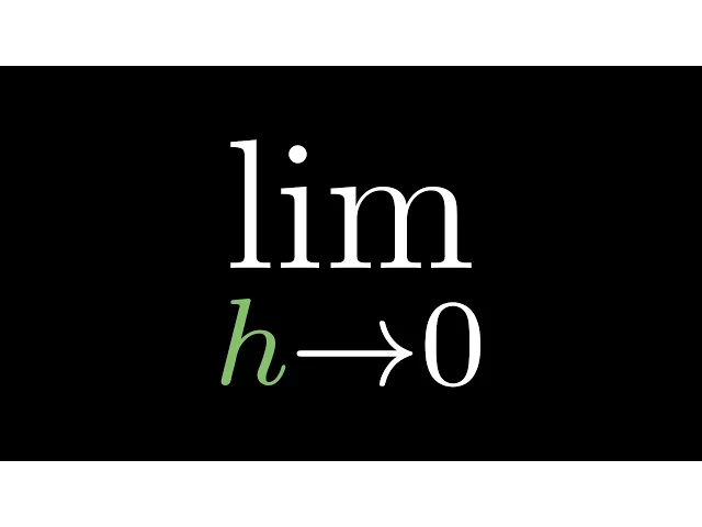
To express that you want to find what this ratio approaches as dx approaches 0,
2:14
you write lim for limit, with dx arrow 0 below it.
2:18
You'll almost never see terms with a lowercase
2:21
d like dx inside a limit expression like this.
2:25
Instead, the standard is to use a different variable,
2:28
something like delta x, or commonly h for whatever reason.
2:31
The way I like to think of it is that terms with this lowercase
2:35
d in the typical derivative expression have built into them this idea of a limit,
2:40
the idea that dx is supposed to eventually go to 0.
2:44
In a sense, this left hand side here, df over dx,
2:47
the ratio we've been thinking about for the past few videos,
2:51
is just shorthand for what the right hand side here spells out in more detail,
2:55
writing out exactly what we mean by df, and writing out this limit process explicitly.
3:01
This right hand side here is the formal definition of a derivative,
3:05
as you would commonly see it in any calculus textbook.
3:08
And if you'll pardon me for a small rant here,
3:11
I want to emphasize that nothing about this right hand side references the paradoxical
3:15
idea of an infinitely small change.
3:18
The point of limits is to avoid that.
3:20
This value h is the exact same thing as the dx
3:23
I've been referencing throughout the series.
3:25
It's a nudge to the input of f with some non-zero, finitely small size, like 0.001.
3:33
It's just that we're analyzing what happens for arbitrarily small choices of h.
3:38
In fact, the only reason people introduce a new variable name into this formal
3:43
definition, rather than just using dx, is to be extra clear that these changes
3:48
to the input are just ordinary numbers that have nothing to do with infinitesimals.
3:54
There are others who like to interpret this dx as an infinitely small change,
3:59
whatever Or to just say that dx and df are nothing more than
4:02
symbols that we shouldn't take too seriously.
4:06
But by now in the series, you know I'm not really a fan of either of those views.
4:10
I think you can and should interpret dx as a concrete, finitely small nudge,
4:14
just so long as you remember to ask what happens when that thing approaches 0.
4:19
For one thing, and I hope the past few videos have helped convince you of this,
4:23
that helps to build stronger intuition for where the rules of calculus actually come from.
4:27
But it's not just some trick for building intuitions.
4:30
Everything I've been saying about derivatives with this concrete,
4:34
finitely small nudge philosophy is just a translation of this formal definition we're
4:38
staring at right now.
4:41
Long story short, the big fuss about limits is that they let us
4:44
avoid talking about infinitely small changes by instead asking what
4:48
happens as the size of some small change to our variable approaches 0.
4:53
And this brings us to goal number 2, understanding
4:56
exactly what it means for one value to approach another.
5:00
For example, consider the function 2 plus h cubed minus 2 cubed all divided by h.
5:08
This happens to be the expression that pops out when you unravel
5:12
the definition of a derivative of x cubed evaluated at x equals 2,
5:16
but let's just think of it as any old function with an input h.
5:20
Its graph is this nice continuous looking parabola,
5:23
which would make sense because it's a cubic term divided by a linear term.
5:28
But actually, if you think about what's going on at h equals 0,
5:32
plugging that in you would get 0 divided by 0, which is not defined.
5:37
So really, this graph has a hole at that point,
5:40
and you have to exaggerate to draw that hole, often with an empty circle like this.
5:45
But keep in mind, the function is perfectly well
5:47
defined for inputs as close to 0 as you want.
5:51
Wouldn't you agree that as h approaches 0, the corresponding output,
5:55
the height of this graph, approaches 12?
5:59
It doesn't matter which side you come at it from.
6:03
That limit of this ratio as h approaches 0 is equal to 12.
6:09
But imagine you're a mathematician inventing calculus,
6:12
and someone skeptically asks you, well, what exactly do you mean by approach?
6:18
That would be kind of an annoying question, I mean, come on,
6:21
we all know what it means for one value to get closer to another.
6:24
But let's start thinking about ways you might be able to answer that person,
6:28
completely unambiguously.
6:30
For a given range of inputs within some distance of 0,
6:34
excluding the forbidden point 0 itself, look at all of the corresponding outputs,
6:39
all possible heights of the graph above that range.
6:42
As the range of input values closes in more and more tightly around 0,
6:47
that range of output values closes in more and more closely around 12.
6:52
And importantly, the size of that range of output values can be made as small as you want.
6:59
As a counter example, consider a function that looks like this,
7:02
which is also not defined at 0, but kind of jumps up at that point.
7:06
When you approach h equals 0 from the right, the function approaches the value 2,
7:11
but as you come at it from the left, it approaches 1.
7:15
Since there's not a single clear, unambiguous value that this function
7:20
approaches as h approaches 0, the limit is not defined at that point.
7:25
One way to think of this is that when you look at any range of inputs around 0,
7:30
and consider the corresponding range of outputs, as you shrink that input range,
7:35
the corresponding outputs don't narrow in on any specific value.
7:39
Instead, those outputs straddle a range that never shrinks smaller than 1,
7:43
even as you make that input range as tiny as you could imagine.
7:48
This perspective of shrinking an input range around the limiting point,
7:52
and seeing whether or not you're restricted in how much that shrinks the output range,
7:56
leads to something called the epsilon-delta definition of limits.
8:01
Now I should tell you, you could argue that this is
8:03
needlessly heavy duty for an introduction to calculus.
8:06
Like I said, if you know what the word approach means,
8:08
you already know what a limit means, there's nothing new on the conceptual level here.
8:12
But this is an interesting glimpse into the field of real analysis,
8:16
and gives you a taste for how mathematicians make the intuitive ideas of calculus more
8:21
airtight and rigorous.
8:23
You've already seen the main idea here.
8:25
When a limit exists, you can make this output range as small as you want,
8:29
but when the limit doesn't exist, that output range cannot get smaller than some
8:33
particular value, no matter how much you shrink the input range around the limiting input.
8:39
Let's freeze that same idea a little more precisely,
8:42
maybe in the context of this example where the limiting value was 12.
8:46
Think about any distance away from 12, where for some reason it's
8:50
common to use the Greek letter epsilon to denote that distance.
8:53
The intent here is that this distance epsilon is as small as you want.
8:58
What it means for the limit to exist is that you will always be able to find a
9:04
range of inputs around our limiting point, some distance delta around 0,
9:10
so that any input within delta of 0 corresponds to an output within a distance
9:16
epsilon of 12.
9:18
The key point here is that that's true for any epsilon,
9:21
no matter how small, you'll always be able to find the corresponding delta.
9:25
In contrast, when a limit does not exist, as in this example here,
9:29
you can find a sufficiently small epsilon, like 0.4,
9:33
so that no matter how small you make your range around 0, no matter how tiny delta is,
9:39
the corresponding range of outputs is just always too big.
9:43
There is no limiting output where everything is within a distance epsilon of that output.
9:54
So far, this is all pretty theory-heavy, don't you think?
9:57
Limits being used to formally define the derivative,
10:00
and epsilons and deltas being used to rigorously define the limit itself.
10:04
So let's finish things off here with a trick for actually computing limits.
10:09
For instance, let's say for some reason you were studying
10:12
the function sin of pi times x divided by x squared minus 1.
10:16
Maybe this was modeling some kind of dampened oscillation.
10:20
When you plot a bunch of points to graph this, it looks pretty continuous.
10:27
But there's a problematic value at x equals 1.
10:30
When you plug that in, sin of pi is 0, and the denominator also comes out to 0,
10:35
so the function is actually not defined at that input,
10:39
and the graph should have a hole there.
10:42
This also happens at x equals negative 1, but let's just
10:45
focus our attention on a single one of these holes for now.
10:50
The graph certainly does seem to approach a distinct value at that point,
10:53
wouldn't you say?
10:57
So you might ask, how exactly do you find what output this approaches as x approaches 1,
11:03
since you can't just plug in 1?
11:07
Well, one way to approximate it would be to plug in
11:11
a number that's just really close to 1, like 1.00001.
11:16
Doing that, you'd find that this should be a number around negative 1.57.
11:21
But is there a way to know precisely what it is?
11:23
Some systematic process to take an expression like this one,
11:27
that looks like 0 divided by 0 at some input, and ask what is its limit as x
11:32
approaches that input?
11:36
After limits, so helpfully let us write the definition for derivatives,
11:40
derivatives can actually come back here and return the favor to help us evaluate limits.
11:45
Let me show you what I mean.
11:47
Here's what the graph of sin of pi times x looks like,
11:50
and here's what the graph of x squared minus 1 looks like.
11:53
That's a lot to have up on the screen, but just
11:56
focus on what's happening around x equals 1.
12:00
The point here is that sin of pi times x and x squared minus 1 are both 0 at that point,
12:06
they both cross the x axis.
12:09
In the same spirit as plugging in a specific value near 1, like 1.00001,
12:14
let's zoom in on that point and consider what happens just a tiny nudge dx away from it.
12:21
The value sin of pi times x is bumped down, and the value of that nudge,
12:26
which was caused by the nudge dx to the input, is what we might call d sin of pi x.
12:33
And from our knowledge of derivatives, using the chain rule,
12:37
that should be around cosine of pi times x times pi times dx.
12:42
Since the starting value was x equals 1, we plug in x equals 1 to that expression.
12:51
In other words, the amount that this sin of pi times x graph changes is roughly
12:56
proportional to dx, with a proportionality constant equal to cosine of pi times pi.
13:03
And cosine of pi, if we think back to our trig knowledge,
13:06
is exactly negative 1, so we can write this whole thing as negative pi times dx.
13:12
Similarly, the value of the x squared minus 1 graph changes by some dx squared minus 1,
13:18
and taking the derivative, the size of that nudge should be 2x times dx.
13:24
Again, we were starting at x equals 1, so we plug in x equals 1 to that expression,
13:29
meaning the size of that output nudge is about 2 times 1 times dx.
13:34
What this means is that for values of x which are just a tiny nudge dx away from 1,
13:41
the ratio sin of pi x divided by x squared minus 1 is approximately
13:46
negative pi times dx divided by 2 times dx.
13:50
The dx's cancel out, so what's left is negative pi over 2.
13:55
And importantly, those approximations get more and more
13:58
accurate for smaller and smaller choices of dx, right?
14:02
This ratio, negative pi over 2, actually tells
14:05
us the precise limiting value as x approaches 1.
14:09
Remember, what that means is that the limiting height on
14:13
our original graph is evidently exactly negative pi over 2.
14:18
What happened there is a little subtle, so I want to go through it again,
14:21
but this time a little more generally.
14:24
Instead of these two specific functions, which are both equal to 0 at x equals 1,
14:29
think of any two functions, f of x and g of x, which are both 0 at some common value,
14:34
x equals a.
14:36
The only constraint is that these have to be functions where you're
14:39
able to take a derivative of them at x equals a,
14:41
which means they each basically look like a line when you zoom in close
14:45
enough to that value.
14:47
Even though you can't compute f divided by g at this trouble point,
14:52
since both of them equal 0, you can ask about this ratio for
14:56
values of x really close to a, the limit as x approaches a.
15:01
It's helpful to think of those nearby inputs as just a tiny nudge, dx, away from a.
15:06
The value of f at that nudged point is approximately its derivative,
15:12
df over dx, evaluated at a times dx.
15:15
Likewise, the value of g at that nudged point is approximately the derivative of g,
15:22
evaluated at a times dx.
15:25
Near that trouble point, the ratio between the outputs of f and g is actually about the
15:31
same as the derivative of f at a times dx, divided by the derivative of g at a times dx.
15:37
Those dx's cancel out, so the ratio of f and g near a
15:41
is about the same as the ratio between their derivatives.
15:45
Because each of those approximations gets more and more accurate for smaller and
15:50
smaller nudges, this ratio of derivatives gives the precise value for the limit.
15:55
This is a really handy trick for computing a lot of limits.
15:58
Whenever you come across some expression that seems to equal 0 divided by
16:02
0 when you plug in some particular input, just try taking the derivative
16:06
of the top and bottom expressions and plugging in that same trouble input.
16:13
This clever trick is called L'Hopital's Rule.
16:17
Interestingly, it was actually discovered by Johann Bernoulli,
16:20
but L'Hopital was this wealthy dude who essentially paid
16:22
Bernoulli for the rights to some of his mathematical discoveries.
16:26
Academia is weird back then, but in a very literal way,
16:30
it pays to understand these tiny nudges.
16:34
Right now, you might be remembering that the definition of a derivative
16:38
for a given function comes down to computing the limit of a certain
16:42
fraction that looks like 0 divided by 0, so you might think that
16:45
L'Hopital's Rule could give us a handy way to discover new derivative formulas.
16:50
But that would actually be cheating, since presumably
16:53
you don't know what the derivative of the numerator is.
16:57
When it comes to discovering derivative formulas,
16:59
something we've been doing a fair amount this series,
17:02
there is no systematic plug-and-chug method.
17:05
But that's a good thing!
17:06
Whenever creativity is needed to solve problems like these,
17:09
it's a good sign that you're doing something real,
17:11
something that might give you a powerful tool to solve future problems.
17:18
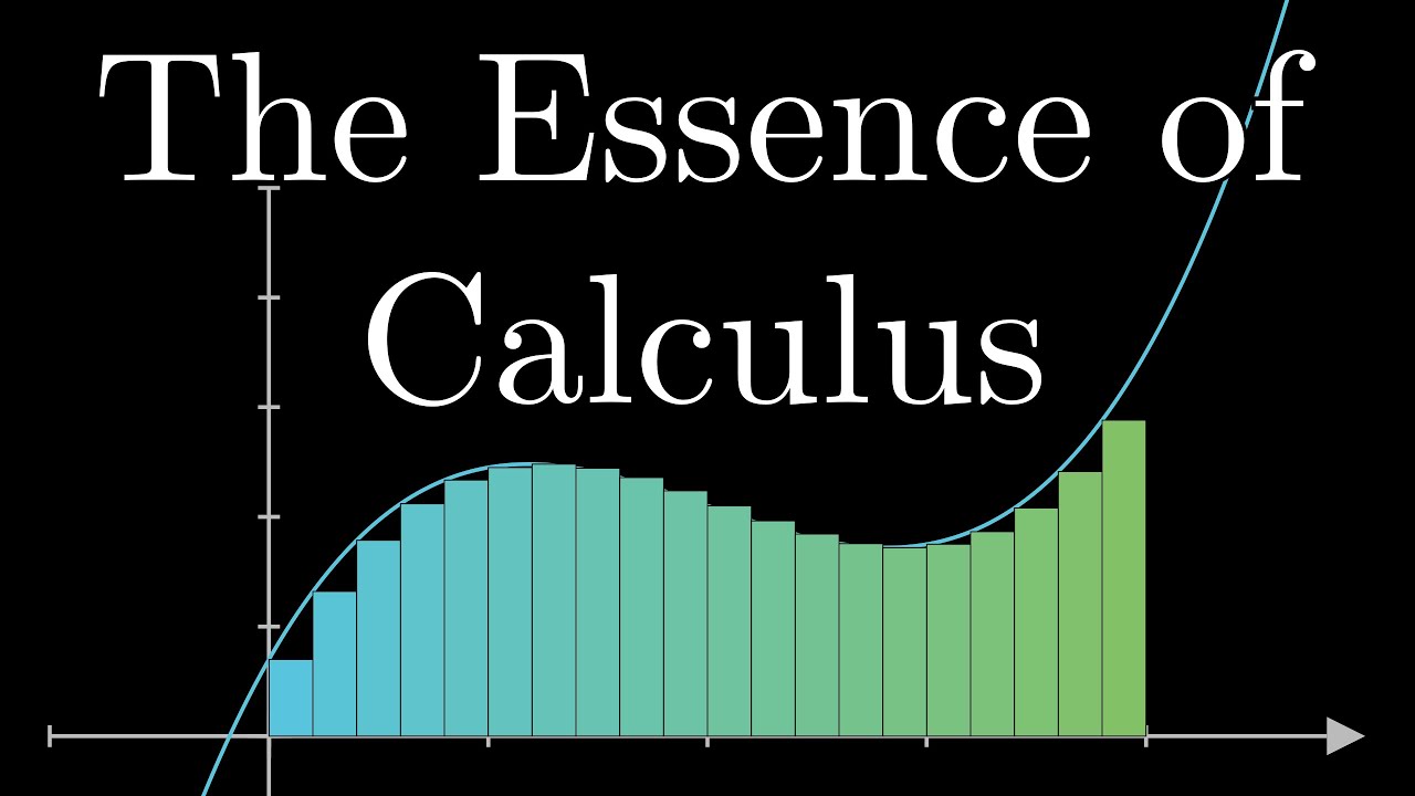
And speaking of powerful tools, up next I'm going to be talking about what an integral
17:22
is, as well as the fundamental theorem of calculus,
17:25
another example of where limits can be used to give a clear meaning to a pretty delicate
17:30
idea that flirts with infinity.
17:33
As you know, most support for this channel comes through Patreon,
17:36
and the primary perk for patrons is early access to future series like this one,
17:40
where the next one is going to be on probability.
17:44
But for those of you who want a more tangible way to flag that
17:47
you're part of the community, there is also a small 3blue1brown store.
17:52
Links on the screen and in the description.
17:54
I'm still debating whether or not to make a preliminary batch of plushie pie creatures,
18:05
it depends on how many viewers seem interested in the store more generally,
18:14
but let me know in comments what other kinds of things you'd like to see in there.
18:23
Thanks for watching!
— end of transcript —
Advertisement