Advertisement
 14:26
14:26
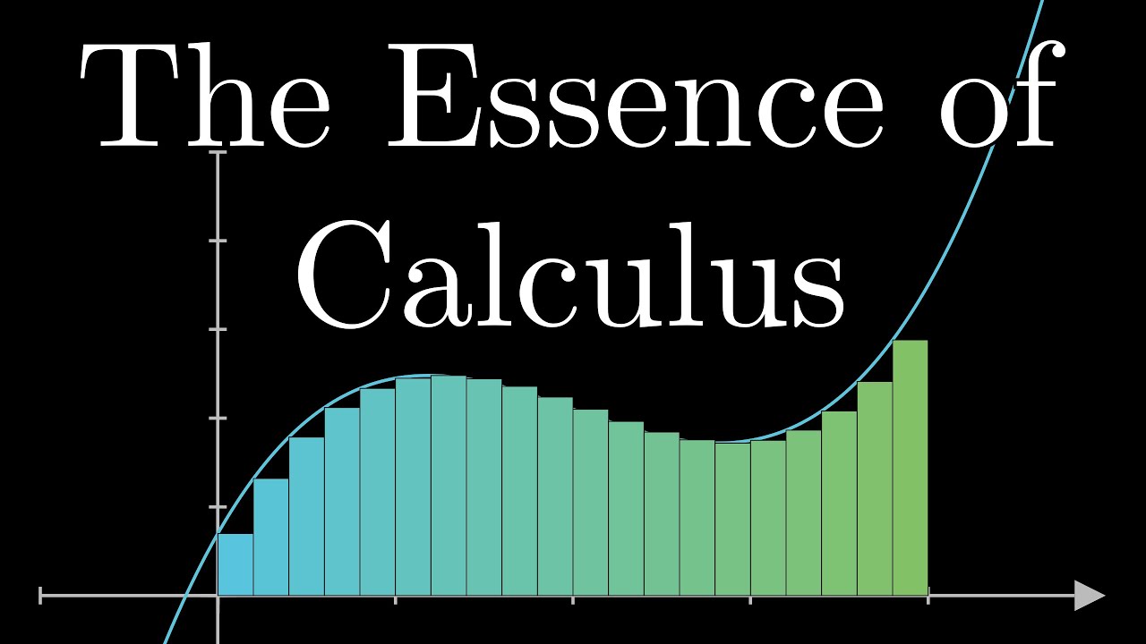
The other way to visualize derivatives | Chapter 12, Essence of calculus
3Blue1Brown
·
May 12, 2026
Open on YouTube
Transcript
0:07
The months ahead of you hold within them a lot of hard work, some neat examples,
0:11
some not-so-neat examples, beautiful connections to physics,
0:14
not-so-beautiful piles of formulas to memorize,
0:17
plenty of moments of getting stuck and banging your head into a wall,
0:20
a few nice aha moments sprinkled in as well, and some genuinely lovely
0:24
graphical intuition to help guide you through it all.
0:27
But if the course ahead of you is anything like my first introduction to calculus,
0:31
or any of the first courses I've seen in the years since,
Advertisement
0:34
there's one topic you will not see, but which I believe stands to greatly accelerate
0:38
your learning.
0:40
You see, almost all of the visual intuitions from that first year are based on graphs.
0:45
The derivative is the slope of a graph, the integral is a certain area under that graph.
0:50
But as you generalize calculus beyond functions whose inputs and outputs are
0:54
simply numbers, it's not always possible to graph the function you're analyzing.
1:00
So if all your intuitions for the fundamental ideas, like derivatives,
1:04
are rooted too rigidly in graphs, it can make for a very tall and largely
1:08
unnecessary conceptual hurdle between you and the more quote-unquote advanced
1:13
topics like multivariable calculus and complex analysis, differential geometry.
Advertisement
1:18
What I want to share with you is a way to think about derivatives,
1:22
which I'll refer to as the transformational view,
1:24
that generalizes more seamlessly into some of those more general contexts
1:28
where calculus comes up.
1:29
And then we'll use this alternate view to analyze a fun puzzle about repeated fractions.
1:35
But first off, I just want to make sure we're all
1:37
on the same page about what the standard visual is.
1:40
If you were to graph a function, which simply takes real numbers as inputs and outputs,
1:44
one of the first things you learn in a calculus course is that the derivative gives
1:49
you the slope of this graph, where what we mean by that is that the derivative of
1:54
the function is a new function which for every input x returns that slope.
1:59
Now I'd encourage you not to think of this derivative
2:01
as slope idea as being the definition of a derivative.
2:05
Instead think of it as being more fundamentally about how
2:07
sensitive the function is to tiny little nudges around the input.
2:11
And the slope is just one way to think about that sensitivity
2:14
relevant only to this particular way of viewing functions.
2:17
I have not just another video, but a full series on this
2:19
topic if it's something you want to learn more about.
2:22
The basic idea behind the alternate visual for the derivative is to
2:26
think of this function as mapping all of the input points on the
2:29
number line to their corresponding outputs on a different number line.
2:33
In this context, what the derivative gives you is a measure of how
2:36
much the input space gets stretched or squished in various regions.
2:41
That is, if you were to zoom in around a specific input and take a look at some
2:46
evenly spaced points around it, the derivative of the function of that input is
2:51
going to tell you how spread out or contracted those points become after the mapping.
2:57
Here, a specific example helps.
2:59
Take the function x2, it maps 1 to 1, 2 to 4, 3 to 9, and so on.
3:06
You can also see how it acts on all of the points in between.
3:12
If you were to zoom in on a little cluster of points around the input 1,
3:16
and see where they land around the relevant output,
3:19
which for this function also happens to be 1, you'd notice that they tend
3:23
to get stretched out.
3:25
In fact, it roughly looks like stretching out by a factor of 2.
3:29
The closer you zoom in, the more this local behavior looks just like multiplying by a
3:35
factor of 2. This is what it means for the derivative of x2 at the input x equals 1 to be
3:41
2.
3:42
It's what that fact looks like in the context of transformations.
3:46
If you looked at a neighborhood of points around the input 3,
3:49
they would get stretched out by a factor of 6.
3:52
This is what it means for the derivative of this function at the input 3 to equal 6.
3:58
Around the input 1 fourth, a small region tends to get contracted specifically by a
4:03
factor of 1 half, and that's what it looks like for a derivative to be smaller than 1.
4:10
The input 0 is interesting.
4:13
Zooming in by a factor of 10, it doesn't really
4:15
look like a constant stretching or squishing.
4:18
For one thing, all of the outputs end up on the right positive side of things.
4:23
As you zoom in closer and closer, by 100x, or by 1000x,
4:27
it looks more and more like a small neighborhood of points around 0 just
4:33
gets collapsed into 0 itself. This is what it looks like for the derivative to be 0.
4:40
The local behavior looks more and more like multiplying the whole number line by 0.
4:45
It doesn't have to completely collapse everything to a point at a particular zoom level,
4:49
instead it's a matter of what the limiting behavior is as you zoom in closer and closer.
4:55
It's also instructive to take a look at the negative inputs here.
5:00
Things start to feel a little cramped since they collide with where all the positive
5:04
input values go, and this is one of the downsides of thinking of functions as
5:08
transformations.
5:09
But for derivatives, we only really care about the local behavior anyway,
5:13
what happens in a small range around a given input.
5:16
Here, notice that the inputs in a little neighborhood around, say,
5:20
negative 2, don't just get stretched out, they also get flipped around.
5:24
Specifically, the action on such a neighborhood looks more
5:28
and more like multiplying by negative 4 the closer you zoom in.
5:32
This is what it looks like for the derivative of a function to be negative.
5:38
And I think you get the point, this is all well and good,
5:40
but let's see how this is actually useful in solving a problem.
5:44
A friend of mine recently asked me a pretty fun question about the infinite
5:48
fraction 1 plus 1 divided by 1 plus 1 divided by 1 plus 1 divided by 1,
5:52
and clearly you watch math videos online, so maybe you've seen this before,
5:56
but my friend's question actually cuts to something you might not have
5:59
thought about before, relevant to the view of derivatives we're looking at here.
6:05
The typical way you might evaluate an expression like this is to set it equal to x,
6:09
and then notice that there is a copy of the full fraction inside itself.
6:14
So you can replace that copy with another x, and then just solve for x.
6:19
That is, what you want is to find a fixed point of the function 1 plus 1 divided by x.
6:27
But here's the thing, there are actually two solutions for x,
6:30
two special numbers where 1 plus 1 divided by that number gives you back the same thing.
6:36
One is the golden ratio, phi, around 1.618, and the other is negative 0.618,
6:42
which happens to be negative 1 divided by phi.
6:46
I like to call this other number phi's little brother,
6:49
since just about any property that phi has, this number also has.
6:53
And this raises the question, would it be valid to say that the infinite
6:58
fraction we saw is somehow also equal to phi's little brother, negative 0.618?
7:04
Maybe you initially say, obviously not, everything on the left hand side is positive,
7:08
so how could it possibly equal a negative number?
7:12
Well, first we should be clear about what we actually mean by an expression like this.
7:17
One way you could think about it, and it's not the only way,
7:21
there's freedom for choice here, is to imagine starting with some constant, like 1,
7:26
and then repeatedly applying the function 1 plus 1 divided by x, and then asking,
7:30
what is this approach as you keep going?
7:36
I mean, certainly symbolically what you get looks more and more
7:38
like our infinite fraction, so maybe if you wanted to equal a number,
7:41
you should ask what this series of numbers approaches.
7:45
And if that's your view of things, maybe you start off with a negative number,
7:48
so it's not so crazy for the whole expression to end up negative.
7:52
After all, if you start with negative 1 divided by phi,
7:55
then applying this function 1 plus 1 over x, you get back the same number,
7:59
negative 1 divided by phi, so no matter how many times you apply it,
8:03
you're staying fixed at this value.
8:07
But even then, there is one reason you should
8:10
view phi as the favorite brother in this pair.
8:14
Here, try this, pull up a calculator of some kind, then start with any random number,
8:19
and plug it into this function, 1 plus 1 divided by x,
8:22
and plug that number into 1 plus 1 over x, and again, and again, and again, and again.
8:28
No matter what constant you start with, you eventually end up at 1.618.
8:33
Even if you start with a negative number, even one that's really close to phi's
8:38
little brother, eventually it shies away from that value and jumps back over to phi.
8:50
So, what's going on here?
8:52
Why is one of these fixed points favored above the other one?
8:56
Maybe you can already see how the transformational understanding of derivatives
9:00
is helpful for understanding this setup, but for the sake of having a point of contrast,
9:03
I want to show you how a problem like this is often taught using graphs.
9:07
If you were to plug in some random input to this function,
9:11
the y value tells you the corresponding output, right?
9:14
So to think about plugging that output back into the function,
9:17
you might first move horizontally until you hit the line y equals x,
9:22
and that's going to give you a position where the x value corresponds to your
9:26
previous y value, right?
9:28
So then from there, you can move vertically to see what output this new x value has,
9:34
and then you repeat.
9:36
You move horizontally to the line y equals x to find a point whose x value is the same
9:40
as the output you just got, and then you move vertically to apply the function again.
9:45
Now personally, I think this is kind of an awkward way
9:48
to think about repeatedly applying a function, don't you?
9:51
I mean, it makes sense, but you kind of have to pause
9:53
and think about it to remember which way to draw the lines.
9:57
And you can, if you want, think through what conditions make this spiderweb
10:01
process narrow in on a fixed point, versus propagating away from it.
10:05
In fact, go ahead, pause right now, and try to think it through as an exercise.
10:09
It has to do with slopes.
10:12
Or if you want to skip the exercise for something that I think gives a much more
10:15
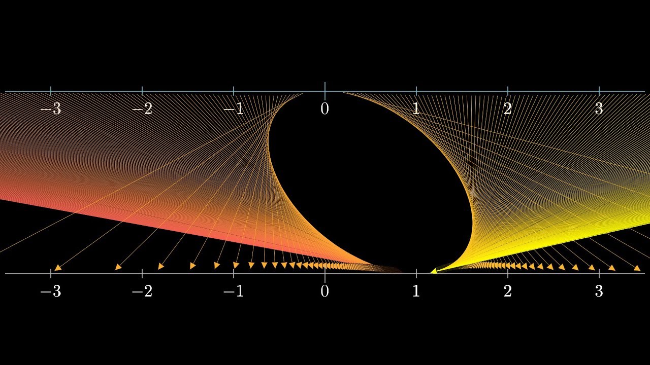
satisfying understanding, think about how this function acts as a transformation.
10:22
So I'm going to go ahead and start here by drawing a bunch of
10:24
arrows to indicate where the various sampled input points will go.
10:28
And side note, don't you think this gives a neat emergent pattern?
10:31
I wasn't expecting this, but it was cool to see it pop up when animating.
10:35
I guess the action of 1 divided by x gives this nice emergent circle,
10:38
and then we're just shifting things over by 1.
10:42
Anyway, I want you to think about what it means to repeatedly apply some function,
10:46
like 1 plus 1 over x, in this context.
10:50
Well after letting it map all of the inputs to the outputs,
10:53
you could consider those as the new inputs, and then just apply the same process again,
10:58
and then again, and do it however many times you want.
11:02
Notice, in animating this with a few dots representing the sample points,
11:06
it doesn't take many iterations at all before all of those dots kind of clump in around 1.
11:11
618.
11:14
Now remember, we know that 1.618 and its little brother,
11:18
negative 0.618 on and on, stay fixed in place during each iteration of this process.
11:24
But zoom in on a neighborhood around phi.
11:27
During the map, points in that region get contracted around phi,
11:32
meaning that the function 1 plus 1 over x has a derivative with a magnitude less
11:39
than 1 at this input.
11:41
In fact, this derivative works out to be around negative 0.38.
11:46
So what that means is that each repeated application scrunches the neighborhood
11:50
around this number smaller and smaller, like a gravitational pull towards phi.
11:54
So now tell me what you think happens in the neighborhood of phi's little brother.
12:01
Over there, the derivative actually has a magnitude larger than 1,
12:05
so points near the fixed point are repelled away from it.
12:09
And when you work it out, you can see that they get
12:11
stretched by more than a factor of 2 in each iteration.
12:14
They also get flipped around, because the derivative is negative here,
12:17
but the salient fact for the sake of stability is just the magnitude.
12:23
Mathematicians would call this right value a stable fixed point,
12:26
and the left one is an unstable fixed point.
12:30
Something is considered stable if when you perturb it just a little bit,
12:33
it tends to come back towards where it started, rather than going away from it.
12:38
So what we're seeing is a very useful little fact,
12:40
that the stability of a fixed point is determined by whether or not the magnitude of its
12:45
derivative is bigger or smaller than 1.
12:47
This explains why phi always shows up in the numerical play,
12:50
where you're just hitting enter on your calculator over and over,
12:53
but phi's little brother never does.
12:56
As to whether or not you want to consider phi's little brother a
12:59
valid value of the infinite fraction, well that's really up to you.
13:03
Everything we just showed suggests that if you think of this expression
13:06
as representing a limiting process, then because every possible seed
13:10
value other than phi's little brother gives you a series converging to phi,
13:14
it does feel silly to put them on equal footing with each other.
13:18
But maybe you don't think of it as a limit, maybe the kind of math
13:21
you're doing lends itself to treating this as a purely algebraic object,
13:25
like the solutions of a polynomial, which simply has multiple values.
13:30
Anyway, that's beside the point, and my point here is not that viewing derivatives
13:34
as this change in density is somehow better than the graphical intuition on the whole.
13:39
In fact, picturing an entire function this way can be
13:42
kind of clunky and impractical as compared to graphs.
13:45
My point is that it deserves more of a mention in most of the
13:48
introductory calculus courses, because it can help make a
13:50
student's understanding of the derivative a little more flexible.
13:54
Like I mentioned, the real reason I'd recommend you carry this perspective
13:58
with you as you learn new topics is not so much for what it does with your
14:01
understanding of single variable calculus, it's for what comes after.
— end of transcript —
Advertisement