Advertisement
 16:50
16:50
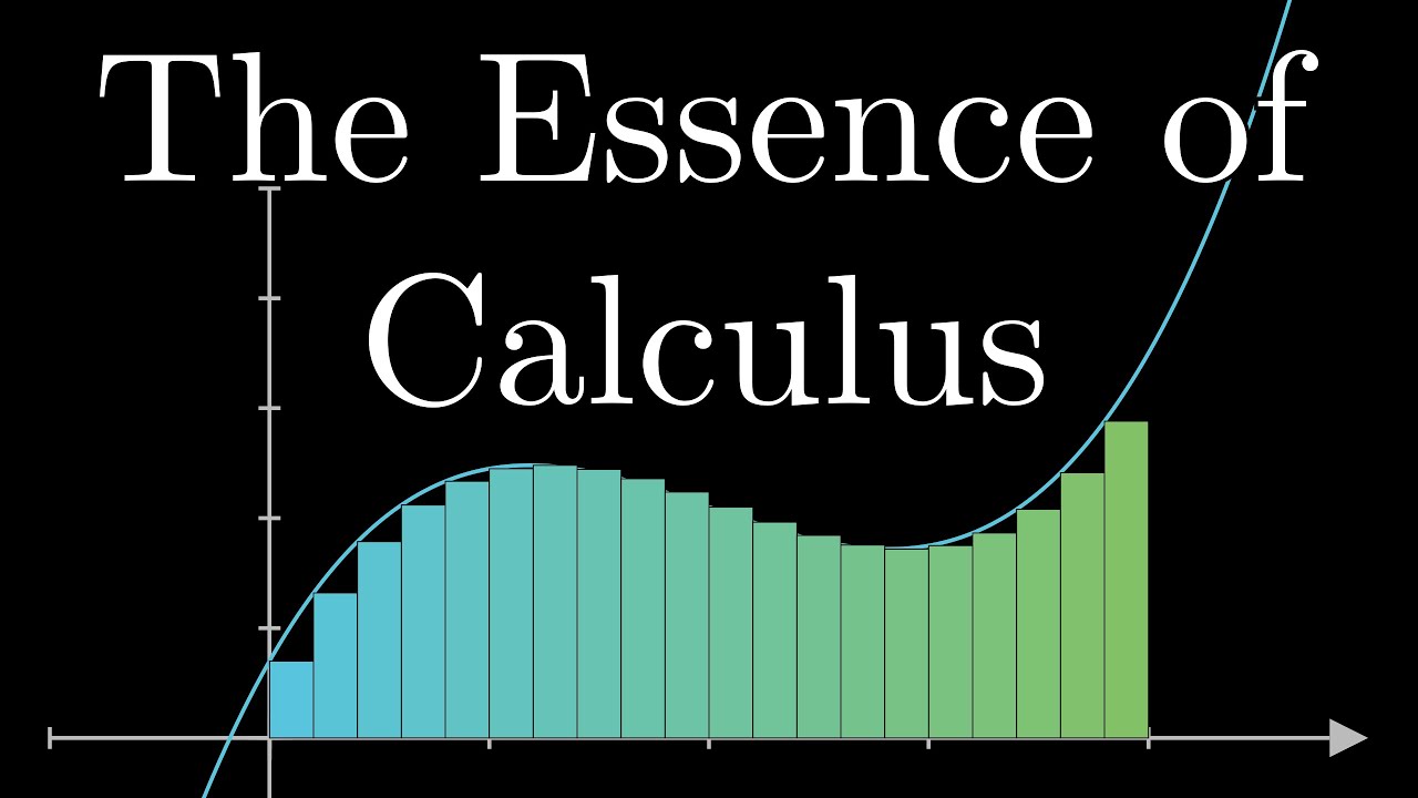
The paradox of the derivative | Chapter 2, Essence of calculus
3Blue1Brown
·
May 12, 2026
Open on YouTube
Transcript
0:15
The goal here is simple, explain what a derivative is.
0:19
The thing is though, there's some subtlety to this topic,
0:21
and a lot of potential for paradoxes if you're not careful.
0:24
So a secondary goal is that you have an appreciation
0:27
for what those paradoxes are and how to avoid them.
0:31
You see, it's common for people to say that the derivative measures an instantaneous
0:35
rate of change, but when you think about it, that phrase is actually an oxymoron.
0:40
Change is something that happens between separate points in time,
Advertisement
0:43
and when you blind yourself to all but just a single instant,
0:46
there's not really any room for change.
0:49
You'll see what I mean more as we get into it,
0:51
but when you appreciate that a phrase like instantaneous rate of change is actually
0:56
nonsense, I think it makes you appreciate just how clever the fathers of calculus
1:00
were in capturing the idea that phrase is meant to evoke,
1:02
but with a perfectly sensible piece of math, the derivative.
1:07
As our central example, I want you to imagine a car that starts at some point A,
1:11
speeds up, and then slows down to a stop at some point B 100 meters away,
1:15
and let's say it all happens over the course of 10 seconds.
Advertisement
1:20
That's the setup to have in mind as we lay out what the derivative is.
1:23
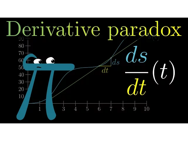
Well, we could graph this motion, letting the vertical axis represent the
1:29
distance traveled, and the horizontal axis represent time, so at each time t,
1:34
represented with a point somewhere on the horizontal axis,
1:38
the height of the graph tells us how far the car has traveled in total after
1:44
that amount of time.
1:46
It's pretty common to name a distance function like this s of t.
1:50
I would use the letter d for distance, but that
1:52
guy already has another full time job in calculus.
1:56
Initially, the curve is quite shallow, since the car is slow to start.
2:00
During that first second, the distance it travels doesn't change that much.
2:04
For the next few seconds, as the car speeds up,
2:07
the distance traveled in a given second gets larger,
2:10
which corresponds to a steeper slope in this graph.
2:13
Then towards the end, when it slows down, that curve shallows out again.
2:20
If we were to plot the car's velocity in meters per second as a function of time,
2:25
it might look like this bump.
2:27
At early times, the velocity is very small.
2:30
Up to the middle of the journey, the car builds up to some maximum velocity,
2:34
covering a relatively large distance each second.
2:37
Then it slows back down towards a speed of zero.
2:41
These two curves are definitely related to each other.
2:44
If you change the specific distance vs.
2:47
time function, you'll have some different velocity vs.
2:50
time function.
2:51
What we want to understand is the specifics of that relationship.
2:55
Exactly how does velocity depend on a distance vs.
2:59
time function?
3:01
To do that, it's worth taking a moment to think
3:04
critically about what exactly velocity means here.
3:08
Intuitively, we all might know what velocity at a given moment means,
3:11
it's just whatever the car's speedometer shows in that moment.
3:17
Intuitively, it might make sense that the car's velocity should be higher at times when
3:21
this distance function is steeper, when the car traverses more distance per unit time.
3:26
But the funny thing is, velocity at a single moment makes no sense.
3:31
If I show you a picture of a car, just a snapshot in an instant,
3:34
and I ask you how fast it's going, you'd have no way of telling me.
3:39
What you'd need are two separate points in time to compare.
3:43
That way you can compute whatever the change in distance across those times is,
3:47
divided by the change in time.
3:49
Right?
3:49
I mean, that's what velocity is, it's the distance traveled per unit time.
3:55
So how is it that we're looking at a function for velocity that
3:59
only takes in a single value of t, a single snapshot in time?
4:02
It's weird, isn't it?
4:04
We want to associate individual points in time with a velocity,
4:07
but actually computing velocity requires comparing two separate points in time.
4:14
If that feels strange and paradoxical, good!
4:17
You're grappling with the same conflicts that the fathers of calculus did.
4:21
And if you want a deep understanding for rates of change, not just for a moving car,
4:25
but for all sorts of things in science, you're going to need to resolve this apparent
4:29
paradox.
4:32
First, I think it's best to talk about the real world,
4:34
and then we'll go into a purely mathematical one.
4:37
Let's think about what the car's speedometer is probably doing.
4:41
At some point, say 3 seconds into the journey,
4:43
the speedometer might measure how far the car goes in a very small amount of time,
4:48
maybe the distance traveled between 3 seconds and 3.01 seconds.
4:53
Then it could compute the speed in meters per second as that tiny
4:57
distance traversed in meters divided by that tiny time, 0.01 seconds.
5:02
That is, a physical car just side-steps the paradox and
5:05
doesn't actually compute speed at a single point in time.
5:08
It computes speed during a very small amount of time.
5:13
So let's call that difference in time dt, which you might think of as 0.01 seconds,
5:18
and let's call that resulting difference in distance ds.
5:22
So the velocity at some point in time is ds divided by dt,
5:26
the tiny change in distance over the tiny change in time.
5:31
Graphically, you can imagine zooming in on some point of this distance vs.
5:35
time graph above t equals 3.
5:38
That dt is a small step to the right, since time is on the horizontal axis,
5:43
and that ds is the resulting change in the height of the graph,
5:47
since the vertical axis represents the distance traveled.
5:51
So ds divided by dt is something you can think of as the rise
5:55
over run slope between two very close points on this graph.
6:00
Of course, there's nothing special about the value t equals 3.
6:03
We could apply this to any other point in time,
6:06
so we consider this expression ds over dt to be a function of t,
6:10
something where I can give you a time t and you can give me back the value of this
6:15
ratio at that time, the velocity as a function of time.
6:19
For example, when I had the computer draw this bump curve here,
6:22
the one representing the velocity function, here's what I had the computer actually do.
6:27
First, I chose a small value for dt, I think in this case it was 0.01.
6:33
Then I had the computer look at a whole bunch of times t between 0 and 10,
6:38
and compute the distance function s at t plus dt,
6:41
and then subtract off the value of that function at t.
6:45
In other words, that's the difference in the distance traveled between the given time,
6:51
t, and the time 0.01 seconds after that.
6:54
Then you can just divide that difference by the change in time, dt,
6:58
and that gives you velocity in meters per second around each point in time.
7:04
So with a formula like this, you could give the computer any curve representing any
7:08
distance function s of t, and it could figure out the curve representing velocity.
7:13
Now would be a good time to pause, reflect, and make sure this idea
7:17
of relating distance to velocity by looking at tiny changes makes sense,
7:21
because we're going to tackle the paradox of the derivative head on.
7:27
This idea of ds over dt, a tiny change in the value of the function s divided by
7:32
the tiny change in the input that caused it, that's almost what a derivative is.
7:38
And even though a car's speedometer will actually look at a concrete change in time,
7:43
like 0.01 seconds, and even though the drawing program here is looking at an actual
7:49
concrete change in time, in pure math the derivative is not this ratio ds over dt for a
7:54
specific choice of dt. Instead, it's whatever that ratio approaches as your choice for dt
7:59
approaches 0.
8:02
Luckily there is a really nice visual understanding for what it means to ask what
8:07
this ratio approaches, Remember, for any specific choice of dt,
8:11
this ratio ds over dt is the slope of a line passing through two separate points
8:15
on the graph, right?
8:17
Well as dt approaches 0, and as those two points approach each other,
8:22
the slope of the line approaches the slope of a line that's
8:26
tangent to the graph at whatever point t we're looking at.
8:30
So the true honest-to-goodness pure math derivative is not the
8:33
rise over run slope between two nearby points on the graph,
8:37
it's equal to the slope of a line tangent to the graph at a single point.
8:42
Now notice what I'm not saying, I'm not saying that the derivative is
8:45
whatever happens when dt is infinitely small, whatever that would mean.
8:50
Nor am I saying that you plug in 0 for dt.
8:53
This dt is always a finitely small non-zero value, it's just that it approaches 0 is all.
9:03
I think that's really clever.
9:05
Even though change in an instant makes no sense,
9:08
this idea of letting dt approach 0 is a really sneaky backdoor
9:12
way to talk reasonably about the rate of change at a single point in time.
9:17
Isn't that neat?
9:18
It's kind of flirting with the paradox of change in
9:20
an instant without ever needing to actually touch it.
9:23
And it comes with such a nice visual intuition too,
9:25
as the slope of a tangent line to a single point on the graph.
9:30
And because change in an instant still makes no sense,
9:33
I think it's healthiest for you to think of this slope not as some instantaneous
9:37
rate of change, but instead as the best constant approximation for a rate of
9:41
change around a point.
9:44
By the way, it's worth saying a couple words on notation here.
9:47
Throughout this video I've been using dt to refer to a tiny change in t with
9:51
some actual size, and ds to refer to the resulting change in s,
9:55
which again has an actual size, and this is because that's how I want you to
9:59
think about them.
10:01
But the convention in calculus is that whenever you're using the letter d like this,
10:05
you're kind of announcing your intention that eventually you're
10:08
going to see what happens as dt approaches 0.
10:11
For example, the honest-to-goodness pure math derivative is written as ds divided by dt,
10:16
even though it's technically not a fraction per se,
10:19
but whatever that fraction approaches for smaller and smaller nudges in t.
10:25
I think a specific example should help here.
10:28
You might think that asking about what this ratio approaches
10:31
for smaller and smaller values would make it much more difficult to compute,
10:35
but weirdly it kind of makes things easier.
10:38
Let's say you have a given distance vs time function that happens to be exactly t cubed.
10:43
So after 1 second the car has traveled 1 cubed equals 1 meters,
10:47
after 2 seconds it's traveled 2 cubed, or 8 meters, and so on.
10:53
Now what I'm about to do might seem somewhat complicated,
10:55
but once the dust settles it really is simpler,
10:57
and more importantly it's the kind of thing you only ever have to do once in calculus.
11:03
Let's say you wanted to compute the velocity, ds divided by dt,
11:06
at some specific time, like t equals 2.
11:09
For right now let's think of dt as having an actual size,
11:13
some concrete nudge, we'll let it go to 0 in just a bit.
11:17
The tiny change in distance between 2 seconds and 2 plus dt
11:22
seconds is s of 2 plus dt minus s of 2, and we divide that by dt.
11:28
Since our function is t cubed, that numerator looks like 2 plus dt cubed minus 2 cubed.
11:35
And this is something we can work out algebraically.
11:38
Again, bear with me, there's a reason I'm showing you the details here.
11:42
When you expand that top, what you get is 2 cubed plus 3 times 2 squared dt
11:49
plus 3 times 2 times dt squared plus dt cubed, and all of that is minus 2 cubed.
11:58
Now there's a lot of terms, and I want you to remember that it looks like a mess,
12:01
but it does simplify.
12:03
Those 2 cubed terms cancel out.
12:06
Everything remaining here has a dt in it, and since there's a dt on the bottom there,
12:11
many of those cancel out as well.
12:14
What this means is that the ratio ds divided by dt has boiled down into
12:19
3 times 2 squared plus 2 different terms that each have a dt in them.
12:25
So if we ask what happens as dt approaches 0, representing the idea of looking at a
12:30
smaller and smaller change in time, we can just completely ignore those other terms.
12:36
By eliminating the need to think about a specific dt,
12:39
we've eliminated a lot of the complication in the full expression.
12:43
So what we're left with is this nice clean 3 times 2 squared.
12:48
You can think of that as meaning that the slope of a line tangent to
12:52
the point at t equals 2 of this graph is exactly 3 times 2 squared, or 12.
12:57
And of course, there's nothing special about the time t equals 2.
13:01
We could more generally say that the derivative
13:04
of t cubed as a function of t is 3 times t squared.
13:10
Now take a step back, because that's beautiful.
13:13
The derivative is this crazy complicated idea.
13:16
We've got tiny changes in distance over tiny changes in time,
13:19
but instead of looking at any specific one of those,
13:22
we're talking about what that thing approaches.
13:24
I mean, that's a lot to think about.
13:27
And yet what we've come out with is such a simple expression, 3 times t squared.
13:32
And in practice, you wouldn't go through all this algebra each time.
13:36
Knowing that the derivative of t cubed is 3t squared is one of those things that all
13:40
calculus students learn how to do immediately without having to re-derive it each time.
13:45
And in the next video, I'm going to show you a nice way to think about
13:48
this and a couple other derivative formulas in really nice geometric ways.
13:52
But the point I want to make by showing you all of the algebraic guts
13:56
here is that when you consider the tiny change in distance caused by a
14:00
tiny change in time for some specific value of dt, you'd have kind of a mess.
14:05
But when you consider what that ratio approaches as dt approaches 0,
14:08
it lets you ignore much of that mess, and it really does simplify the problem.
14:13
That right there is kind of the heart of why calculus becomes useful.
14:18
Another reason to show you a concrete derivative like this is that it
14:21
sets the stage for an example of the kind of paradoxes that come about
14:25
if you believe too much in the illusion of instantaneous rate of change.
14:30
So think about the actual car traveling according to this t cubed distance function,
14:34
and consider its motion at the moment t equals 0, right at the start.
14:39
Now ask yourself whether or not the car is moving at that time.
14:45
On the one hand, we can compute its speed at that point using the derivative,
14:50
3t squared, which for time t equals 0 works out to be 0.
14:54
Visually, this means that the tangent line to the graph at that point is perfectly flat,
14:59
so the car's quote-unquote instantaneous velocity is 0,
15:03
and that suggests that obviously it's not moving.
15:07
But on the other hand, if it doesn't start moving at time 0, when does it start moving?
15:12
Really, pause and ponder that for a moment.
15:15
Is the car moving at time t equals 0?
15:22
Do you see the paradox?
15:24
The issue is that the question makes no sense.
15:26
It references the idea of change in a moment, but that doesn't actually exist.
15:30
That's just not what the derivative measures.
15:33
What it means for the derivative of a distance function to be 0 is that the best
15:38
constant approximation for the car's velocity around that point is 0 m per second.
15:44
For example, if you look at an actual change in time,
15:47
say between time 0 and 0.1 seconds, the car does move.
15:51
It moves 0.001 m.
15:54
That's very small, and importantly, it's very small compared to the change in time,
15:59
giving an average speed of only 0.01 m per second.
16:03
And remember, what it means for the derivative of this motion to be 0 is that
16:08
for smaller and smaller nudges in time, this ratio of m per second approaches 0.
16:14
But that's not to say that the car is static.
16:17
Approximating its movement with a constant velocity of 0 is,
16:20
after all, just an approximation.
16:24
So whenever you hear people refer to the derivative as an instantaneous rate of change,
16:29
a phrase which is intrinsically oxymoronic, I want you to think of that as a
16:33
conceptual shorthand for the best constant approximation for rate of change.
16:39
In the next couple videos, I'll be talking more about the derivative,
16:42
what it looks like in different contexts, how do you actually compute it,
16:45
why is it useful, things like that, focusing on visual intuition as always.
— end of transcript —
Advertisement