Advertisement
 22:19
22:19
Transcript
0:14
When I first learned about Taylor series, I definitely
0:17
didn't appreciate just how important they are.
0:20
But time and time again they come up in math, physics,
0:22
and many fields of engineering because they're one of the most
0:25
powerful tools that math has to offer for approximating functions.
0:30
I think one of the first times this clicked for me as a
0:32
student was not in a calculus class but a physics class.
0:35
We were studying a certain problem that had to do with the potential energy of a
Advertisement
0:40
pendulum, and for that you need an expression for how high the weight of the
0:44
pendulum is above its lowest point, and when you work that out it comes out to be
0:48
proportional to 1 minus the cosine of the angle between the pendulum and the vertical.
0:53
The specifics of the problem we were trying to solve are beyond the point here,
0:57
but what I'll say is that this cosine function made the problem awkward and unwieldy,
1:02
and made it less clear how pendulums relate to other oscillating phenomena.
1:07
But if you approximate cosine of theta as 1 minus theta squared over 2,
1:12
everything just fell into place much more easily.
1:16
If you've never seen anything like this before,
1:19
an approximation like that might seem completely out of left field.
Advertisement
1:23
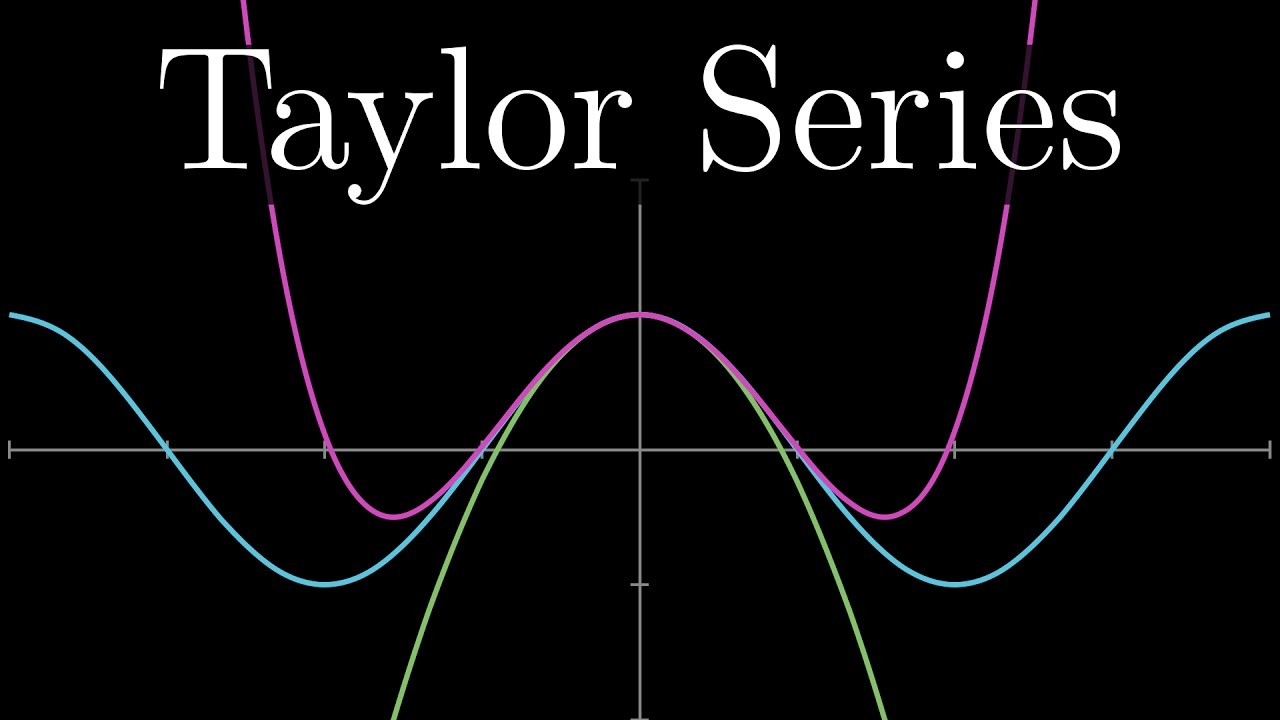
If you graph cosine of theta along with this function, 1 minus theta squared over 2,
1:28
they do seem rather close to each other, at least for small angles near 0,
1:33
but how would you even think to make this approximation,
1:36
and how would you find that particular quadratic?
1:41
The study of Taylor series is largely about taking non-polynomial
1:44
functions and finding polynomials that approximate them near some input.
1:48
The motive here is that polynomials tend to be much easier to deal
1:52
with than other functions, they're easier to compute,
1:55
easier to take derivatives, easier to integrate, just all around more friendly.
2:00
So let's take a look at that function, cosine of x,
2:03
and really take a moment to think about how you might construct a quadratic
2:08
approximation near x equals 0.
2:10
That is, among all of the possible polynomials that look like c0 plus c1
2:16
times x plus c2 times x squared, for some choice of these constants, c0,
2:21
c1, and c2, find the one that most resembles cosine of x near x equals 0,
2:27
whose graph kind of spoons with the graph of cosine x at that point.
2:33
Well, first of all, at the input 0, the value of cosine of x is 1,
2:38
so if our approximation is going to be any good at all,
2:41
it should also equal 1 at the input x equals 0.
2:45
Plugging in 0 just results in whatever c0 is, so we can set that equal to 1.
2:53
This leaves us free to choose constants c1 and c2 to make this
2:56
approximation as good as we can, but nothing we do with them is
3:00
going to change the fact that the polynomial equals 1 at x equals 0.
3:04
It would also be good if our approximation had the same
3:08
tangent slope as cosine x at this point of interest.
3:11
Otherwise the approximation drifts away from the
3:14
cosine graph much faster than it needs to.
3:18
The derivative of cosine is negative sine, and at x equals 0,
3:22
that equals 0, meaning the tangent line is perfectly flat.
3:26
On the other hand, when you work out the derivative of our quadratic,
3:31
you get c1 plus 2 times c2 times x.
3:35
At x equals 0, this just equals whatever we choose for c1.
3:40
So this constant c1 has complete control over the
3:43
derivative of our approximation around x equals 0.
3:47
Setting it equal to 0 ensures that our approximation
3:49
also has a flat tangent line at this point.
3:53
This leaves us free to change c2, but the value and the slope of our
3:57
polynomial at x equals 0 are locked in place to match that of cosine.
4:04
The final thing to take advantage of is the fact that the cosine graph
4:08
curves downward above x equals 0, it has a negative second derivative.
4:13
Or in other words, even though the rate of change is 0 at that point,
4:17
the rate of change itself is decreasing around that point.
4:21
Specifically, since its derivative is negative sine of x,
4:25
its second derivative is negative cosine of x, and at x equals 0, that equals negative 1.
4:33
Now in the same way that we wanted the derivative of our approximation to
4:37
match that of the cosine so that their values wouldn't drift apart needlessly quickly,
4:41
making sure that their second derivatives match will ensure that they
4:45
curve at the same rate, that the slope of our polynomial doesn't drift
4:49
away from the slope of cosine x any more quickly than it needs to.
4:54
Pulling up the same derivative we had before, and then taking its derivative,
4:59
we see that the second derivative of this polynomial is exactly 2 times c2.
5:04
So to make sure that this second derivative also equals negative 1 at x equals 0,
5:10
2 times c2 has to be negative 1, meaning c2 itself should be negative 1 half.
5:16
This gives us the approximation 1 plus 0x minus 1 half x squared.
5:23
To get a feel for how good it is, if you estimate cosine of 0.1 using this polynomial,
5:29
you'd estimate it to be 0.995, and this is the true value of cosine of 0.1.
5:36
It's a really good approximation!
5:40
Take a moment to reflect on what just happened.
5:42
You had 3 degrees of freedom with this quadratic approximation,
5:46
the constants c0, c1, and c2.
5:49
c0 was responsible for making sure that the output of the approximation matches that of
5:55
cosine x at x equals 0, c1 was in charge of making sure that the derivatives match at
6:01
that point, and c2 was responsible for making sure that the second derivatives match up.
6:08
This ensures that the way your approximation changes as you move away from x equals 0,
6:14
and the way that the rate of change itself changes,
6:17
is as similar as possible to the behaviour of cosine x,
6:20
given the amount of control you have.
6:24
You could give yourself more control by allowing more terms
6:27
in your polynomial and matching higher order derivatives.
6:30
For example, let's say you added on the term c3 times x cubed for some constant c3.
6:36
In that case, if you take the third derivative of a cubic polynomial,
6:41
anything quadratic or smaller goes to 0.
6:45
As for that last term, after 3 iterations of the power rule,
6:50
it looks like 1 times 2 times 3 times c3.
6:56
On the other hand, the third derivative of cosine x comes out to sine x,
7:01
which equals 0 at x equals 0.
7:03
So to make sure that the third derivatives match, the constant c3 should be 0.
7:09
Or in other words, not only is 1 minus ½ x2 the best possible quadratic
7:14
approximation of cosine, it's also the best possible cubic approximation.
7:21
You can make an improvement by adding on a fourth order term, c4 times x to the fourth.
7:27
The fourth derivative of cosine is itself, which equals 1 at x equals 0.
7:34
And what's the fourth derivative of our polynomial with this new term?
7:38
Well, when you keep applying the power rule over and over,
7:42
with those exponents all hopping down in front,
7:45
you end up with 1 times 2 times 3 times 4 times c4, which is 24 times c4.
7:51
So if we want this to match the fourth derivative of cosine x,
7:56
which is 1, c4 has to be 1 over 24.
7:59
And indeed, the polynomial 1 minus ½ x2 plus 1 24 times x to the fourth,
8:05
which looks like this, is a very close approximation for cosine x around x equals 0.
8:13
In any physics problem involving the cosine of a small angle, for example,
8:18
predictions would be almost unnoticeably different if you substituted this polynomial
8:23
for cosine of x.
8:26
Take a step back and notice a few things happening with this process.
8:30
First of all, factorial terms come up very naturally in this process.
8:35
When you take n successive derivatives of the function x to the n,
8:39
letting the power rule keep cascading on down,
8:43
what you'll be left with is 1 times 2 times 3 on and on up to whatever n is.
8:49
So you don't simply set the coefficients of the polynomial equal to whatever derivative
8:53
you want, you have to divide by the appropriate factorial to cancel out this effect.
8:59
For example, that x to the fourth coefficient was the fourth derivative of cosine,
9:05
1, but divided by 4 factorial, 24.
9:09
The second thing to notice is that adding on new terms,
9:12
like this c4 times x to the fourth, doesn't mess up what the old terms should be,
9:17
and that's really important.
9:20
For example, the second derivative of this polynomial at x equals 0 is still equal
9:25
to 2 times the second coefficient, even after you introduce higher order terms.
9:30
And it's because we're plugging in x equals 0,
9:33
so the second derivative of any higher order term, which all include an x,
9:38
will just wash away.
9:40
And the same goes for any other derivative, which is why each derivative of a
9:45
polynomial at x equals 0 is controlled by one and only one of the coefficients.
9:52
If instead you were approximating near an input other than 0, like x equals pi,
9:57
in order to get the same effect you would have to write your polynomial in
10:01
terms of powers of x minus pi, or whatever input you're looking at.
10:06
This makes it look noticeably more complicated,
10:09
but all we're doing is making sure that the point pi looks and behaves like 0,
10:13
so that plugging in x equals pi will result in a lot of nice cancellation that
10:18
leaves only one constant.
10:22
And finally, on a more philosophical level, notice how what we're doing here is basically
10:27
taking information about higher order derivatives of a function at a single point,
10:32
and translating that into information about the value of the function near that point.
10:40
You can take as many derivatives of cosine as you want.
10:44
It follows this nice cyclic pattern, cosine of x,
10:47
negative sine of x, negative cosine, sine, and then repeat.
10:52
And the value of each one of these is easy to compute at x equals 0.
10:56
It gives this cyclic pattern 1, 0, negative 1, 0, and then repeat.
11:02
And knowing the values of all those higher order derivatives is a lot of information
11:07
about cosine of x, even though it only involves plugging in a single number, x equals 0.
11:14
So what we're doing is leveraging that information to get an approximation around this
11:19
input, and you do it by creating a polynomial whose higher order derivatives are designed
11:25
to match up with those of cosine, following this same 1, 0, negative 1, 0, cyclic pattern.
11:31
And to do that, you just make each coefficient of the polynomial follow that
11:35
same pattern, but you have to divide each one by the appropriate factorial.
11:40
Like I mentioned before, this is what cancels out
11:42
the cascading effect of many power rule applications.
11:47
The polynomials you get by stopping this process at
11:50
any point are called Taylor polynomials for cosine of x.
11:53
More generally, and hence more abstractly, if we were dealing with some other function
11:58
other than cosine, you would compute its derivative, its second derivative, and so on,
12:03
getting as many terms as you'd like, and you would evaluate each one of them at x equals
12:08
0.
12:09
Then for the polynomial approximation, the coefficient of each x to the n term should be
12:15
the value of the nth derivative of the function evaluated at 0,
12:20
but divided by n factorial.
12:23
This whole rather abstract formula is something you'll likely
12:27
see in any text or course that touches on Taylor polynomials.
12:31
And when you see it, think to yourself that the constant term ensures that
12:36
the value of the polynomial matches with the value of f,
12:39
the next term ensures that the slope of the polynomial matches the slope
12:43
of the function at x equals 0, the next term ensures that the rate at which
12:48
the slope changes is the same at that point, and so on,
12:51
depending on how many terms you want.
12:54
And the more terms you choose, the closer the approximation,
12:57
but the tradeoff is that the polynomial you'd get would be more complicated.
13:02
And to make things even more general, if you wanted to approximate near some input
13:07
other than 0, which we'll call a, you would write this polynomial in terms of powers
13:12
of x minus a, and you would evaluate all the derivatives of f at that input, a.
13:18
This is what Taylor polynomials look like in their fullest generality.
13:24
Changing the value of a changes where this approximation is hugging the original
13:28
function, where its higher order derivatives will be equal to those of the original
13:33
function.
13:35
One of the simplest meaningful examples of this is
13:38
the function e to the x around the input x equals 0.
13:42
Computing the derivatives is super nice, as nice as it gets,
13:46
because the derivative of e to the x is itself,
13:49
so the second derivative is also e to the x, as is its third, and so on.
13:54
So at the point x equals 0, all of these are equal to 1.
13:59
And what that means is our polynomial approximation should look like
14:05
1 plus 1 times x plus 1 over 2 times x squared plus 1 over 3 factorial times x cubed,
14:13
and so on, depending on how many terms you want.
14:19
These are the Taylor polynomials for e to the x.
14:26
Ok, so with that as a foundation, in the spirit of showing you just how connected all
14:31
the topics of calculus are, let me turn to something kind of fun,
14:34
a completely different way to understand this second order term of the Taylor
14:38
polynomials, but geometrically.
14:41
It's related to the fundamental theorem of calculus,
14:43
which I talked about in chapters 1 and 8 if you need a quick refresher.
14:47
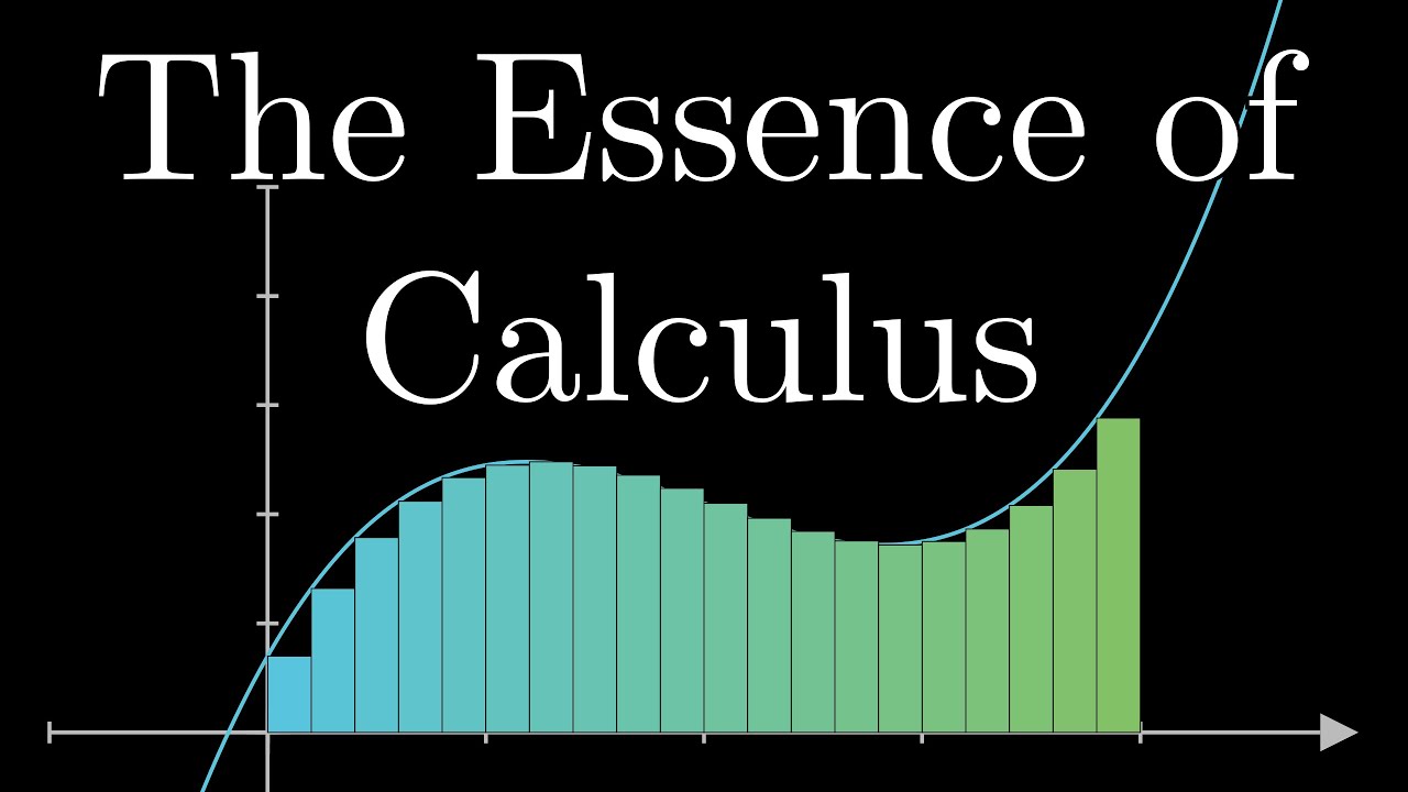
Like we did in those videos, consider a function that gives the area
14:52
under some graph between a fixed left point and a variable right point.
14:56
What we're going to do here is think about how to approximate this area function,
15:00
not the function for the graph itself, like we've been doing before.
15:04
Focusing on that area is what's going to make the second order term pop out.
15:10
Remember, the fundamental theorem of calculus is that this graph itself represents the
15:16
derivative of the area function, and it's because a slight nudge dx to the right bound
15:22
of the area gives a new bit of area approximately equal to the height of the graph times
15:28
dx.
15:30
And that approximation is increasingly accurate for smaller and smaller choices of dx.
15:35
But if you wanted to be more accurate about this change in area,
15:39
given some change in x that isn't meant to approach 0,
15:42
you would have to take into account this portion right here,
15:46
which is approximately a triangle.
15:49
Let's name the starting input a, and the nudged input above it x, so that change is x-a.
15:58
The base of that little triangle is that change, x-a,
16:02
and its height is the slope of the graph times x-a.
16:08
Since this graph is the derivative of the area function,
16:11
its slope is the second derivative of the area function, evaluated at the input a.
16:18
So the area of this triangle, 1 half base times height,
16:22
is 1 half times the second derivative of this area function, evaluated at a,
16:28
multiplied by x-a2.
16:30
And this is exactly what you would see with a Taylor polynomial.
16:34
If you knew the various derivative information about this area function at the point a,
16:40
how would you approximate the area at the point x?
16:45
Well you have to include all that area up to a, f of a,
16:49
plus the area of this rectangle here, which is the first derivative, times x-a,
16:54
plus the area of that little triangle, which is 1 half times the second derivative,
17:00
times x-a2.
17:02
I really like this, because even though it looks a bit messy all written out,
17:06
each one of the terms has a very clear meaning that you can just point to on the diagram.
17:13
If you wanted, we could call it an end here, and you would have a
17:16
phenomenally useful tool for approximating these Taylor polynomials.
17:21
But if you're thinking like a mathematician, one question you might ask is
17:25
whether or not it makes sense to never stop and just add infinitely many terms.
17:31
In math, an infinite sum is called a series, so even though one of these
17:35
approximations with finitely many terms is called a Taylor polynomial,
17:40
adding all infinitely many terms gives what's called a Taylor series.
17:45
You have to be really careful with the idea of an infinite series,
17:48
because it doesn't actually make sense to add infinitely many things,
17:52
you can only hit the plus button on the calculator so many times.
17:57
But if you have a series where adding more and more of the terms,
18:01
which makes sense at each step, gets you increasingly close to some specific value,
18:06
what you say is that the series converges to that value.
18:10
Or, if you're comfortable extending the definition of equality to
18:14
include this kind of series convergence, you'd say that the series as a whole,
18:19
this infinite sum, equals the value it's converging to.
18:23
For example, look at the Taylor polynomial for e to the x,
18:27
and plug in some input, like x equals 1.
18:31
As you add more and more polynomial terms, the total sum gets closer and
18:36
closer to the value e, so you say that this infinite series converges to the number e,
18:42
or what's saying the same thing, that it equals the number e.
18:47
In fact, it turns out that if you plug in any other value of x, like x equals 2,
18:53
and look at the value of the higher and higher order Taylor polynomials at this value,
18:59
they will converge towards e to the x, which is e squared.
19:04
This is true for any input, no matter how far away from 0 it is,
19:08
even though these Taylor polynomials are constructed only from derivative information
19:14
gathered at the input 0.
19:18
In a case like this, we say that e to the x equals its own Taylor series at all inputs x,
19:24
which is kind of a magical thing to have happen.
19:28
Even though this is also true for a couple other important functions,
19:32
like sine and cosine, sometimes these series only converge within a
19:36
certain range around the input whose derivative information you're using.
19:41
If you work out the Taylor series for the natural log of x around the input x equals 1,
19:47
which is built by evaluating the higher order derivatives of the natural
19:51
log of x at x equals 1, this is what it would look like.
19:56
When you plug in an input between 0 and 2, adding more and more terms of this
20:00
series will indeed get you closer and closer to the natural log of that input.
20:06
But outside of that range, even by just a little bit,
20:09
the series fails to approach anything.
20:12
As you add on more and more terms, the sum bounces back and forth wildly.
20:18
It does not, as you might expect, approach the natural log of that value,
20:22
even though the natural log of x is perfectly well defined for inputs above 2.
20:28
In some sense, the derivative information of ln
20:31
of x at x equals 1 doesn't propagate out that far.
20:36
In a case like this, where adding more terms of the series doesn't approach anything,
20:41
you say that the series diverges.
20:44
And that maximum distance between the input you're approximating
20:47
near and points where the outputs of these polynomials actually
20:51
converge is called the radius of convergence for the Taylor series.
20:56
There remains more to learn about Taylor series.
20:59
There are many use cases, tactics for placing bounds on the error of
21:03
these approximations, tests for understanding when series do and don't converge,
21:07
and for that matter, there remains more to learn about calculus as a whole,
21:11
and the countless topics not touched by this series.
21:15
The goal with these videos is to give you the fundamental intuitions
21:19
that make you feel confident and efficient in learning more on your own,
21:23
and potentially even rediscovering more of the topic for yourself.
21:28
In the case of Taylor series, the fundamental intuition to keep in mind
21:32
as you explore more of what there is, is that they translate derivative
21:36
information at a single point to approximation information around that point.
21:43
Thank you once again to everybody who supported this series.
21:47
The next series like it will be on probability,
21:49
and if you want early access as those videos are made, you know where to go.
22:11
Thank you.
— end of transcript —
Advertisement